You can run this notebook in a live session ![]() or view it on Github.
or view it on Github.
Table of Contents
1 Compare weighted and unweighted mean temperature
1.0.1 Data
1.0.2 Creating weights
1.0.3 Weighted mean
1.0.4 Plot: comparison with unweighted mean
Compare weighted and unweighted mean temperature#
Author: Mathias Hauser
We use the air_temperature example dataset to calculate the area-weighted temperature over its domain. This dataset has a regular latitude/ longitude grid, thus the grid cell area decreases towards the pole. For this grid we can use the cosine of the latitude as proxy for the grid cell area.
[1]:
%matplotlib inline

import cartopy.crs as ccrs
import matplotlib.pyplot as plt
import numpy as np

import xarray as xr
Data#
Load the data, convert to celsius, and resample to daily values
[2]:
ds = xr.tutorial.load_dataset("air_temperature")

# to celsius
air = ds.air - 273.15

# resample from 6-hourly to daily values
air = air.resample(time="D").mean()

air
[2]:
<xarray.DataArray 'air' (time: 730, lat: 25, lon: 53)> Size: 8MB
array([[[-31.2775, -30.85  , -30.475 , ..., -39.7775, -37.975 ,
         -35.475 ],
        [-28.575 , -28.5775, -28.875 , ..., -41.9025, -40.325 ,
         -36.85  ],
        [-19.15  , -19.9275, -21.3275, ..., -41.675 , -39.455 ,
         -34.525 ],
        ...,
        [ 23.15  ,  22.825 ,  22.85  , ...,  22.7475,  22.17  ,
          21.795 ],
        [ 23.175 ,  23.575 ,  23.5925, ...,  23.0225,  22.85  ,
          22.3975],
        [ 23.47  ,  23.845 ,  23.95  , ...,  23.8725,  23.8975,
          23.8225]],

       [[-29.55  , -29.65  , -29.85  , ..., -34.1775, -32.3525,
         -30.0775],
        [-25.3275, -25.95  , -26.9275, ..., -37.225 , -36.5525,
         -34.55  ],
        [-19.6275, -21.0775, -22.8525, ..., -35.4525, -34.2775,
         -31.25  ],
...
        [ 23.215 ,  22.265 ,  22.015 , ...,  23.74  ,  23.195 ,
          22.195 ],
        [ 24.3675,  24.515 ,  23.895 , ...,  23.415 ,  22.995 ,
          22.27  ],
        [ 25.4175,  25.5925,  25.1925, ...,  23.6425,  23.19  ,
          22.72  ]],

       [[-28.935 , -29.535 , -30.385 , ..., -29.41  , -28.96  ,
         -28.46  ],
        [-23.835 , -24.06  , -24.56  , ..., -32.585 , -31.635 ,
         -30.035 ],
        [-10.21  , -10.785 , -11.435 , ..., -33.685 , -31.035 ,
         -27.135 ],
        ...,
        [ 21.69  ,  21.99  ,  23.49  , ...,  22.265 ,  22.015 ,
          21.415 ],
        [ 23.39  ,  24.44  ,  24.94  , ...,  22.415 ,  22.315 ,
          21.64  ],
        [ 24.84  ,  25.59  ,  25.54  , ...,  23.065 ,  22.715 ,
          22.39  ]]], shape=(730, 25, 53))
Coordinates:
  * lat      (lat) float32 100B 75.0 72.5 70.0 67.5 65.0 ... 22.5 20.0 17.5 15.0
  * lon      (lon) float32 212B 200.0 202.5 205.0 207.5 ... 325.0 327.5 330.0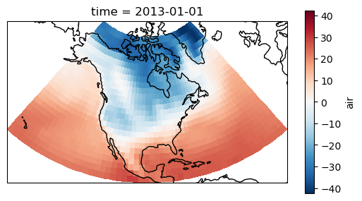
* time (time) datetime64[ns] 6kB 2013-01-01 2013-01-02 ... 2014-12-31Plot the first timestep:
[3]:
projection = ccrs.LambertConformal(central_longitude=-95, central_latitude=45)

f, ax = plt.subplots(subplot_kw=dict(projection=projection))

air.isel(time=0).plot(transform=ccrs.PlateCarree(), cbar_kwargs=dict(shrink=0.7))
ax.coastlines()
[3]:
<cartopy.mpl.feature_artist.FeatureArtist at 0x72fc025d6900>
/home/docs/checkouts/readthedocs.org/user_builds/xray/conda/v2025.10.0/lib/python3.13/site-packages/cartopy/io/__init__.py:242: DownloadWarning: Downloading: https://naturalearth.s3.amazonaws.com/110m_physical/ne_110m_coastline.zip
  warnings.warn(f'Downloading: {url}', DownloadWarning)
Creating weights#
For a rectangular grid the cosine of the latitude is proportional to the grid cell area.
[4]:
weights = np.cos(np.deg2rad(air.lat))
weights.name = "weights"
weights
[4]:
<xarray.DataArray 'weights' (lat: 25)> Size: 100B
array([0.25881907, 0.30070582, 0.34202015, 0.38268346, 0.42261827,
       0.4617486 , 0.49999997, 0.5372996 , 0.57357645, 0.6087614 ,
       0.6427876 , 0.67559016, 0.70710677, 0.7372773 , 0.76604444,
       0.7933533 , 0.81915206, 0.8433914 , 0.8660254 , 0.8870108 ,
       0.90630776, 0.9238795 , 0.9396926 , 0.95371693, 0.9659258 ],
      dtype=float32)
Coordinates:
  * lat      (lat) float32 100B 75.0 72.5 70.0 67.5 65.0 ... 22.5 20.0 17.5 15.0
Attributes:
    standard_name:  latitude
    long_name:      Latitude
    units:          degrees_north
axis: YWeighted mean#
[5]:
air_weighted = air.weighted(weights)
air_weighted
[5]:
DataArrayWeighted with weights along dimensions: lat
[6]:
weighted_mean = air_weighted.mean(("lon", "lat"))
weighted_mean
[6]:
<xarray.DataArray 'air' (time: 730)> Size: 6kB
array([ 6.09242278,  5.52801153,  5.65131014,  5.78625911,  5.91178741,
        5.68345808,  5.97673463,  6.45674666,  6.57108842,  6.50467029,
        6.13492195,  5.92688812,  5.82684419,  5.7228889 ,  5.578026  ,
        5.46554263,  5.09125883,  4.98603299,  5.2286468 ,  5.25168042,
        5.42774537,  5.38781258,  5.43391836,  5.36441932,  5.46855751,
        5.22904788,  5.35030417,  5.34184946,  5.37268972,  5.35953248,
        5.1403546 ,  5.0555833 ,  5.07248201,  5.23523798,  5.31850399,
        5.49919477,  5.72090656,  5.72863393,  5.76082994,  5.82558255,
        6.26852676,  6.43692612,  6.51025574,  6.56479046,  6.60880826,
        6.42129023,  5.9147635 ,  5.55469741,  5.32923554,  5.33592568,
        5.07060741,  5.2837553 ,  5.59523877,  6.0546815 ,  6.53075461,
        6.50744131,  6.3917653 ,  6.39515023,  6.39811177,  6.52939708,
        6.47713445,  6.53578901,  6.69254388,  6.67739312,  6.5116567 ,
        6.44705649,  6.86040296,  7.43756346,  7.69813492,  7.48428983,
        7.25821619,  7.13598516,  7.09343383,  7.26711351,  7.3485635 ,
        7.32181379,  7.22117177,  7.21295352,  7.28406885,  7.54340733,
        7.85440156,  8.11587054,  8.26192767,  8.11165238,  8.21915648,
        8.35874465,  8.71618023,  9.1519191 ,  9.37007869,  9.41590018,
        9.07347135,  8.82068813,  8.80467628,  8.85641443,  9.06748554,
        9.40718574,  9.69696523,  9.7421144 ,  9.65965489,  9.69564904,
...
       17.48434471, 17.33182165, 17.20268511, 17.06828058, 16.91011693,
       16.53698847, 16.13337371, 16.05557413, 16.10014633, 15.90946889,
       15.76415334, 15.63154863, 15.8278093 , 16.02628556, 16.31993632,
       16.15651207, 15.89850898, 15.83092403, 15.81013986, 15.58985426,
       15.30967993, 15.10523434, 14.96473674, 14.96703162, 14.90466044,
       14.61071753, 14.33017104, 14.25566908, 14.31408802, 13.94015833,
       13.75892029, 13.82092018, 14.02188925, 13.88824364, 13.72476435,
       13.19092809, 12.99519974, 12.66989203, 12.58508297, 12.3777192 ,
       12.17870103, 12.08236127, 11.87425249, 11.66021296, 11.60118227,
       11.55865688, 11.18389167, 11.23739079, 11.09196145, 10.472234  ,
        9.89895079,  9.43127566,  9.49163121,  9.68865668,  9.99861322,
        9.79358905,  9.3153213 ,  9.25996986,  9.38503149,  9.34304003,
        9.20262184,  9.47236552,  9.42424866,  9.05071054,  8.56821849,
        7.71917736,  7.33125099,  7.4513287 ,  7.42361835,  7.51882489,
        7.49506521,  7.62389396,  8.08327689,  8.04916245,  8.0273007 ,
        8.06964375,  7.91256129,  8.04297641,  8.34484262,  8.50710337,
        8.7082316 ,  8.60498356,  8.31249645,  8.25727109,  7.98417114,
        7.69333762,  7.42200395,  7.43526565,  7.48298729,  7.64287358,
        7.90849899,  8.03616336,  7.62544799,  7.75334548,  7.85045561,
        7.62133052,  6.84736674,  6.45028939,  5.98526248,  5.58059891])
Coordinates: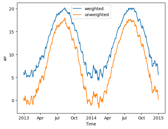
* time (time) datetime64[ns] 6kB 2013-01-01 2013-01-02 ... 2014-12-31Plot: comparison with unweighted mean#
Note how the weighted mean temperature is higher than the unweighted.
[7]:
weighted_mean.plot(label="weighted")
air.mean(("lon", "lat")).plot(label="unweighted")

plt.legend()
[7]:
<matplotlib.legend.Legend at 0x72fc02651be0>