Tutorial
To get started, we will import numpy, pandas and xray:
In [1]: import numpy as np

In [2]: import pandas as pd

In [3]: import xray
Dataset objects
xray.Dataset is xray’s primary data structure. It is a dict-like container of labeled arrays (xray.DataArray objects) with aligned dimensions. It is designed as an in-memory representation of the data model from the NetCDF file format.
Creating a Dataset
To make an xray.Dataset from scratch, pass in a dictionary with values in the form (dimensions, data[, attributes]).
- dimensions should be a sequence of strings.
- data should be a numpy.ndarray (or array-like object) that has a dimensionality equal to the length of the dimensions list.
In [4]: foo_values = np.random.RandomState(0).rand(3, 4)

In [5]: times = pd.date_range('2000-01-01', periods=3)

In [6]: ds = xray.Dataset({'time': ('time', times),
   ...:                    'foo': (['time', 'space'], foo_values)})
   ...:

In [7]: ds
Out[7]:
<xray.Dataset>
Dimensions:     (space: 4, time: 3)
Coordinates:
    space            X
    time                      X
Noncoordinates:
    foo              1        0
Attributes:
    Empty
You can also insert xray.Variable or xray.DataArray objects directly into a Dataset, or create an dataset from a pandas.DataFrame with Dataset.from_dataframe or from a NetCDF file on disk with open_dataset(). See Working with pandas and Serialization and IO.
Dataset contents
Dataset implements the Python dictionary interface, with values given by xray.DataArray objects:
In [8]: 'foo' in ds
Out[8]: True

In [9]: ds.keys()
Out[9]: ['foo', 'time', 'space']

In [10]: ds['time']
Out[10]:
<xray.DataArray 'time' (time: 3)>
array(['1999-12-31T18:00:00.000000000-0600',
       '2000-01-01T18:00:00.000000000-0600',
       '2000-01-02T18:00:00.000000000-0600'], dtype='datetime64[ns]')
Attributes:
    Empty
The valid keys include each listed “coordinate” and “noncoordinate”. Coordinates are arrays that labels values along a particular dimension, which they index by keeping track of a pandas.Index object. They are created automatically from dataset arrays whose name is equal to the one item in their list of dimensions.
Noncoordinates include all arrays in a Dataset other than its coordinates. These arrays can exist along multiple dimensions. The numbers in the columns in the Dataset representation indicate the order in which dimensions appear for each array (on a Dataset, the dimensions are always listed in alphabetical order).
We didn’t explicitly include a coordinate for the “space” dimension, so it was filled with an array of ascending integers of the proper length:
In [11]: ds['space']
Out[11]:
<xray.DataArray 'space' (space: 4)>
array([0, 1, 2, 3])
Attributes:
    Empty

In [12]: ds['foo']
Out[12]:
<xray.DataArray 'foo' (time: 3, space: 4)>
array([[ 0.5488135 ,  0.71518937,  0.60276338,  0.54488318],
       [ 0.4236548 ,  0.64589411,  0.43758721,  0.891773  ],
       [ 0.96366276,  0.38344152,  0.79172504,  0.52889492]])
Attributes:
    Empty
Noncoordinates and coordinates are listed explicitly by the noncoordinates and coordinates attributes.
There are also a few derived variables based on datetime coordinates that you can access from a dataset (e.g., “year”, “month” and “day”), even if you didn’t explicitly add them. These are known as “virtual_variables”:
In [13]: ds['time.dayofyear']
Out[13]:
<xray.DataArray 'time.dayofyear' (time: 3)>
array([1, 2, 3], dtype=int32)
Attributes:
    Empty
Finally, datasets also store arbitrary metadata in the form of attributes:
In [14]: ds.attrs
Out[14]: OrderedDict()

In [15]: ds.attrs['title'] = 'example attribute'

In [16]: ds
Out[16]:
<xray.Dataset>
Dimensions:     (space: 4, time: 3)
Coordinates:
    space            X
    time                      X
Noncoordinates:
    foo              1        0
Attributes:
    title: example attribute
xray does not enforce any restrictions on attributes, but serialization to some file formats may fail if you put in objects that aren’t strings, numbers or arrays.
Modifying datasets
We can update a dataset in-place using Python’s standard dictionary syntax:
In [17]: ds['numbers'] = ('space', [10, 10, 20, 20])

In [18]: ds['abc'] = ('time', ['A', 'B', 'C'])

In [19]: ds
Out[19]:
<xray.Dataset>
Dimensions:     (space: 4, time: 3)
Coordinates:
    space            X
    time                      X
Noncoordinates:
    foo              1        0
    numbers          0
    abc                       0
Attributes:
    title: example attribute
It should be evident now how a Dataset lets you store many arrays along a (partially) shared set of common dimensions and coordinates.
To change the variables in a Dataset, you can use all the standard dictionary methods, including values, items, __del__, get and update.
You also can select and unselect an explicit list of variables by using the select() and unselect() methods to return a new Dataset. select automatically includes the relevant coordinate values:
In [20]: ds.select('abc')
Out[20]:
<xray.Dataset>
Dimensions:     (time: 3)
Coordinates:
    time            X
Noncoordinates:
    abc             0
Attributes:
    title: example attribute
If a coordinate is given as an argument to unselect, it also unselects all variables that use that coordinate:
In [21]: ds.unselect('time', 'space')
Out[21]:
<xray.Dataset>
Dimensions:     ()
Coordinates:
    None
Noncoordinates:
    None
Attributes:
    title: example attribute
You can copy a Dataset by using the copy() method:
In [22]: ds2 = ds.copy()

In [23]: del ds2['time']

In [24]: ds2
Out[24]:
<xray.Dataset>
Dimensions:     (space: 4)
Coordinates:
    space            X
Noncoordinates:
    numbers          0
Attributes:
    title: example attribute
By default, the copy is shallow, so only the container will be copied: the contents of the Dataset will still be the same underlying xray.Variable. You can copy all data by supplying the argument deep=True.
DataArray objects
The contents of a Dataset are DataArray objects, xray’s version of a labeled multi-dimensional array. DataArray supports metadata aware array operations based on their labeled dimensions (axis names) and labeled coordinates (tick values).
The idea of the DataArray is to provide an alternative to pandas.Series and pandas.DataFrame with functionality much closer to standard numpy N-dimensional array. Unlike pandas objects, slicing or manipulating a DataArray always returns another DataArray, and all items in a DataArray must have a single (homogeneous) data type. (To work with heterogeneous data in xray, put separate DataArrays in the same Dataset.)
You create a DataArray by getting an item from a Dataset:
In [25]: foo = ds['foo']

In [26]: foo
Out[26]:
<xray.DataArray 'foo' (time: 3, space: 4)>
array([[ 0.5488135 ,  0.71518937,  0.60276338,  0.54488318],
       [ 0.4236548 ,  0.64589411,  0.43758721,  0.891773  ],
       [ 0.96366276,  0.38344152,  0.79172504,  0.52889492]])
Attributes:
    Empty
Note
You currently cannot make a DataArray without putting objects into Dataset first, unless you use the DataArray.from_series class method to convert an existing pandas.Series. We do intend to define a constructor for making DataArray objects directly in a future version of xray.
Internally, data arrays are uniquely defined by only two attributes:
Like pandas objects, they can be thought of as fancy wrapper around a numpy array:
In [27]: foo.values
Out[27]:
array([[ 0.5488135 ,  0.71518937,  0.60276338,  0.54488318],
       [ 0.4236548 ,  0.64589411,  0.43758721,  0.891773  ],
       [ 0.96366276,  0.38344152,  0.79172504,  0.52889492]])
They also have a tuple of dimension labels:
In [28]: foo.dimensions
Out[28]: ('time', 'space')
They track of their coordinates (tick labels) in a read-only ordered dictionary mapping from dimension names to Coordinate objects:
In [29]: foo.coordinates
Out[29]:
Frozen(OrderedDict([('time', <xray.Coordinate (time: 3)>
array(['1999-12-31T18:00:00.000000000-0600',
       '2000-01-01T18:00:00.000000000-0600',
       '2000-01-02T18:00:00.000000000-0600'], dtype='datetime64[ns]')
Attributes:
    Empty), ('space', <xray.Coordinate (space: 4)>
array([0, 1, 2, 3])
Attributes:
    Empty)]))
They also keep track of their own attributes:
In [30]: foo.attrs
Out[30]: OrderedDict()
You can pull out other variable (including coordinates) from a DataArray’s dataset by indexing the data array with a string:
In [31]: foo['time']
Out[31]:
<xray.DataArray 'time' (time: 3)>
array(['1999-12-31T18:00:00.000000000-0600',
       '2000-01-01T18:00:00.000000000-0600',
       '2000-01-02T18:00:00.000000000-0600'], dtype='datetime64[ns]')
Attributes:
    Empty
Usually, xray automatically manages the Dataset objects that data arrays points to in a satisfactory fashion. For example, it will keep around other dataset variables when possible until there are potential conflicts, such as when you apply a mathematical operation.
However, in some cases, particularly for performance reasons, you may want to explicitly ensure that the dataset only includes the variables you are interested in. For these cases, use the xray.DataArray.select() method to select the names of variables you want to keep around, by default including the name of only the DataArray itself:
In [32]: foo2 = foo.select()

In [33]: foo2
Out[33]:
<xray.DataArray 'foo' (time: 3, space: 4)>
array([[ 0.5488135 ,  0.71518937,  0.60276338,  0.54488318],
       [ 0.4236548 ,  0.64589411,  0.43758721,  0.891773  ],
       [ 0.96366276,  0.38344152,  0.79172504,  0.52889492]])
Attributes:
    Empty
foo2 is generally an equivalent labeled array to foo, but we dropped the dataset variables that are no longer relevant:
In [34]: foo.dataset.keys()
Out[34]: ['foo', 'time', 'space', 'numbers', 'abc']

In [35]: foo2.dataset.keys()
Out[35]: ['time', 'space', 'foo']
Array indexing
Indexing a DataArray works (mostly) just like it does for numpy arrays, except that the returned object is always another DataArray:
In [36]: foo[:2]
Out[36]:
<xray.DataArray 'foo' (time: 2, space: 4)>
array([[ 0.5488135 ,  0.71518937,  0.60276338,  0.54488318],
       [ 0.4236548 ,  0.64589411,  0.43758721,  0.891773  ]])
Attributes:
    Empty

In [37]: foo[0, 0]
Out[37]:
<xray.DataArray 'foo' ()>
array(0.5488135039273248)
Attributes:
    Empty

In [38]: foo[:, [2, 1]]
Out[38]:
<xray.DataArray 'foo' (time: 3, space: 2)>
array([[ 0.60276338,  0.71518937],
       [ 0.43758721,  0.64589411],
       [ 0.79172504,  0.38344152]])
Attributes:
    Empty
xray also supports label based indexing like pandas. Because Coordinate is a thin wrapper around a pandas.Index, label indexing is very fast. To do label based indexing, use the loc attribute:
In [39]: foo.loc['2000-01-01':'2000-01-02', 0]
Out[39]:
<xray.DataArray 'foo' (time: 2)>
array([ 0.5488135,  0.4236548])
Attributes:
    Empty
You can do any of the label indexing operations supported by pandas with the exception of boolean arrays, including looking up particular labels, using slice syntax and using arrays of labels. Like pandas, label based indexing is inclusive of both the start and stop bounds.
Setting values with label based indexing is also supported:
In [40]: foo.loc['2000-01-01', [1, 2]] = -10

In [41]: foo
Out[41]:
<xray.DataArray 'foo' (time: 3, space: 4)>
array([[  0.5488135 , -10.        , -10.        ,   0.54488318],
       [  0.4236548 ,   0.64589411,   0.43758721,   0.891773  ],
       [  0.96366276,   0.38344152,   0.79172504,   0.52889492]])
Attributes:
    Empty
With labeled dimension names, we do not have to rely on dimension order and can use them explicitly to slice data with the indexed() and labeled() methods:
# index by array indices
In [42]: foo.indexed(space=0, time=slice(0, 2))
Out[42]:
<xray.DataArray 'foo' (time: 2)>
array([ 0.5488135,  0.4236548])
Attributes:
    Empty

# index by coordinate labels
In [43]: foo.labeled(time=slice('2000-01-01', '2000-01-02'))
Out[43]:
<xray.DataArray 'foo' (time: 2, space: 4)>
array([[  0.5488135 , -10.        , -10.        ,   0.54488318],
       [  0.4236548 ,   0.64589411,   0.43758721,   0.891773  ]])
Attributes:
    Empty
The arguments to these methods can be any objects that could index the array along that dimension, e.g., labels for an individual value, Python slice objects or 1-dimensional arrays.
We can also use these methods to index all variables in a dataset simultaneously, returning a new dataset:
In [44]: ds.indexed(space=[0], time=[0])
Out[44]:
<xray.Dataset>
Dimensions:     (space: 1, time: 1)
Coordinates:
    space            X
    time                      X
Noncoordinates:
    foo              1        0
    numbers          0
    abc                       0
Attributes:
    title: example attribute
In [45]: ds.labeled(time='2000-01-01')
Out[45]:
<xray.Dataset>
Dimensions:     (space: 4)
Coordinates:
    space            X
Noncoordinates:
    foo              0
    time
    numbers          0
    abc
Attributes:
    title: example attribute
Indexing with xray objects has one important difference from indexing numpy arrays: you can only use one-dimensional arrays to index xray objects, and each indexer is applied “orthogonally” along independent axes, instead of using numpy’s array broadcasting. This means you can do indexing like this, which wouldn’t work with numpy arrays:
In [46]: foo[ds['time.day'] > 1, ds['space'] <= 3]
Out[46]:
<xray.DataArray 'foo' (time: 2, space: 4)>
array([[ 0.4236548 ,  0.64589411,  0.43758721,  0.891773  ],
       [ 0.96366276,  0.38344152,  0.79172504,  0.52889492]])
Attributes:
    Empty
This is a much simpler model than numpy’s advanced indexing, and is basically the only model that works for labeled arrays. If you would like to do advanced indexing, so you always index .values instead:
In [47]: foo.values[foo.values > 0.5]
Out[47]:
array([ 0.5488135 ,  0.54488318,  0.64589411,  0.891773  ,  0.96366276,
        0.79172504,  0.52889492])
DataArray math
The metadata of DataArray objects enables particularly nice features for doing mathematical operations.
Basic math
Basic math works just as you would expect:
In [48]: foo - 3
Out[48]:
<xray.DataArray 'foo___sub___other' (time: 3, space: 4)>
array([[ -2.4511865 , -13.        , -13.        ,  -2.45511682],
       [ -2.5763452 ,  -2.35410589,  -2.56241279,  -2.108227  ],
       [ -2.03633724,  -2.61655848,  -2.20827496,  -2.47110508]])
Attributes:
    Empty
You can also use any of numpy’s or scipy’s many ufunc functions directly on a DataArray:
In [49]: np.sin(foo)
Out[49]:
<xray.DataArray 'foo_' (time: 3, space: 4)>
array([[ 0.52167534,  0.54402111,  0.54402111,  0.51831819],
       [ 0.41109488,  0.60191268,  0.42375525,  0.77818647],
       [ 0.82128673,  0.37411428,  0.71156637,  0.50457956]])
Attributes:
    Empty
Aggregation
Whenever feasible, DataArrays have metadata aware version of standard methods and properties from numpy arrays. For example, we can easily take a metadata aware xray.DataArray.transpose:
In [50]: foo.T
Out[50]:
<xray.DataArray 'foo' (space: 4, time: 3)>
array([[  0.5488135 ,   0.4236548 ,   0.96366276],
       [-10.        ,   0.64589411,   0.38344152],
       [-10.        ,   0.43758721,   0.79172504],
       [  0.54488318,   0.891773  ,   0.52889492]])
Attributes:
    Empty
Most of these methods have been updated to take a dimension argument instead of axis. This allows for very intuitive syntax for aggregation methods that are applied along particular dimension(s):
In [51]: foo.sum('time')
Out[51]:
<xray.DataArray 'foo' (space: 4)>
array([ 1.93613106, -8.97066437, -8.77068775,  1.9655511 ])
Attributes:
    Empty
In [52]: foo.std(['time', 'space'])
Out[52]:
<xray.DataArray 'foo' ()>
array(3.9602436567278514)
Attributes:
    Empty
Currently, these are the standard numpy array methods which do not automatically skip missing values, but we expect to switch to NA skipping versions (like pandas) in the future. For now, you can do NA skipping aggregate by passing NA aware numpy functions to the reduce method:
In [53]: foo.reduce(np.nanmean, 'time')
Out[53]:
<xray.DataArray 'foo' (space: 4)>
array([ 0.64537702, -2.99022146, -2.92356258,  0.6551837 ])
Attributes:
    Empty
If you ever need to figure out the axis number for a dimension yourself (say, for wrapping library code designed to work with numpy arrays), you can use the get_axis_num() method:
In [54]: foo.get_axis_num('space')
Out[54]: 1
Broadcasting
With dimension names, we automatically align dimensions (“broadcasting” in the numpy parlance) by name instead of order. This means that you should never need to bother inserting dimensions of length 1 with operations like np.reshape() or np.newaxis, which is pretty routinely required when working with standard numpy arrays.
This is best illustrated by a few examples. Consider two one-dimensional arrays with different sizes aligned along different dimensions:
In [55]: foo[:, 0]
Out[55]:
<xray.DataArray 'foo' (time: 3)>
array([ 0.5488135 ,  0.4236548 ,  0.96366276])
Attributes:
    Empty

In [56]: foo[0, :]
Out[56]:
<xray.DataArray 'foo' (space: 4)>
array([  0.5488135 , -10.        , -10.        ,   0.54488318])
Attributes:
    Empty
With xray, we can apply binary mathematical operations to arrays, and their dimensions are expanded automatically:
In [57]: foo[:, 0] - foo[0, :]
Out[57]:
<xray.DataArray 'foo___sub___foo' (time: 3, space: 4)>
array([[  0.00000000e+00,   1.05488135e+01,   1.05488135e+01,
          3.93032093e-03],
       [ -1.25158705e-01,   1.04236548e+01,   1.04236548e+01,
         -1.21228384e-01],
       [  4.14849257e-01,   1.09636628e+01,   1.09636628e+01,
          4.18779578e-01]])
Attributes:
    Empty
Moreover, dimensions are always reordered to the order in which they first appeared. That means you can always subtract an array from its transpose!
In [58]: foo - foo.T
Out[58]:
<xray.DataArray 'foo___sub___foo' (time: 3, space: 4)>
array([[ 0.,  0.,  0.,  0.],
       [ 0.,  0.,  0.,  0.],
       [ 0.,  0.,  0.,  0.]])
Attributes:
    Empty
Coordinate based alignment
You can also align arrays based on their coordinate values, very similarly to how pandas handles alignment. This can be done with the reindex() or reindex_like() methods, or the align() top-level function. All these work interchangeably with both DataArray and Dataset objects with any number of overlapping dimensions.
To demonstrate, we’ll make a subset DataArray with new values:
In [59]: bar = (10 * foo[:2, :2]).rename('bar')

In [60]: bar
Out[60]:
<xray.DataArray 'bar' (time: 2, space: 2)>
array([[   5.48813504, -100.        ],
       [   4.23654799,    6.45894113]])
Attributes:
    Empty
Reindexing foo with bar selects out the first two values along each dimension:
In [61]: foo.reindex_like(bar)
Out[61]:
<xray.DataArray 'foo' (time: 2, space: 2)>
array([[  0.5488135 , -10.        ],
       [  0.4236548 ,   0.64589411]])
Attributes:
    Empty
The opposite operation asks us to reindex to a larger shape, so we fill in the missing values with NaN:
In [62]: bar.reindex_like(foo)
Out[62]:
<xray.DataArray 'bar' (time: 3, space: 4)>
array([[   5.48813504, -100.        ,           nan,           nan],
       [   4.23654799,    6.45894113,           nan,           nan],
       [          nan,           nan,           nan,           nan]])
Attributes:
    Empty
The align() is even more flexible:
In [63]: xray.align(ds, bar, join='inner')
Out[63]:
(<xray.Dataset>
 Dimensions:     (space: 2, time: 2)
 Coordinates:
     space            X
     time                      X
 Noncoordinates:
     foo              1        0
     numbers          0
     abc                       0
 Attributes:
     title: example attribute, <xray.DataArray 'bar' (time: 2, space: 2)>
 array([[   5.48813504, -100.        ],
        [   4.23654799,    6.45894113]])
 Attributes:
     Empty)
Pandas does this sort of index based alignment automatically when doing math, using an join=’outer’. This is an intended feature for xray, too, but we haven’t turned it on yet, because it is not clear that an outer join (which preserves all missing values) is the best choice for working with high- dimension arrays. Arguably, an inner join makes more sense, because that is less likely to result in memory blow-ups. Hopefully, this point will eventually become moot when python libraries better support working with arrays that cannot be directly represented in a block of memory.
GroupBy: split-apply-combine
Pandas has very convenient support for “group by” operations, which implement the split-apply-combine strategy for crunching data:
- Split your data into multiple independent groups.
- Apply some function to each group.
- Combine your groups back into a single data object.
xray implements this same pattern using very similar syntax to pandas. Group by operations work on both Dataset and DataArray objects. Note that currently, you can only group by a single one-dimensional variable (eventually, we hope to remove this limitation).
Split
Recall the “numbers” variable in our dataset:
In [64]: ds['numbers']
Out[64]:
<xray.DataArray 'numbers' (space: 4)>
array([10, 10, 20, 20])
Attributes:
    Empty
If we groupby the name of a variable in a dataset (we can also use a DataArray directly), we get back a xray.GroupBy object:
In [65]: ds.groupby('numbers')
Out[65]: <xray.groupby.DatasetGroupBy at 0x6125fd0>
This object works very similarly to a pandas GroupBy object. You can view the group indices with the groups attribute:
In [66]: ds.groupby('numbers').groups
Out[66]: {10: [0, 1], 20: [2, 3]}
You can also iterate over over groups in (label, group) pairs:
In [67]: list(ds.groupby('numbers'))
Out[67]:
[(10, <xray.Dataset>
  Dimensions:     (space: 2, time: 3)
  Coordinates:
      space            X
      time                      X
  Noncoordinates:
      foo              1        0
      numbers          0
      abc                       0
  Attributes:
      title: example attribute), (20, <xray.Dataset>
  Dimensions:     (space: 2, time: 3)
  Coordinates:
      space            X
      time                      X
  Noncoordinates:
      foo              1        0
      numbers          0
      abc                       0
  Attributes:
      title: example attribute)]
Just like in pandas, creating a GroupBy object doesn’t actually split the data until you want to access particular values.
Apply
To apply a function to each group, you can use the flexible xray.GroupBy.apply method. The resulting objects are automatically concatenated back together along the group axis:
In [68]: def standardize(x):
   ....:     return (x - x.mean()) / x.std()
   ....:

In [69]: foo.groupby('numbers').apply(standardize)
Out[69]:
<xray.DataArray 'foo___sub___foo___div___foo' (time: 3, space: 4)>
array([[ 0.43549756, -2.23350501, -2.23430669,  0.42314949],
       [ 0.4038306 ,  0.46006036,  0.39610942,  0.51057051],
       [ 0.54046043,  0.39365606,  0.48535704,  0.41912022]])
Attributes:
    Empty
Group by objects resulting from DataArrays also have shortcuts to aggregate a function over each element of the group:
In [70]: foo.groupby('numbers').mean()
Out[70]:
<xray.DataArray 'foo' (numbers: 2)>
array([-1.17242222, -1.13418944])
Attributes:
    Empty
Squeezing
When grouping over a dimension, you can control whether the dimension is squeezed out or if it should remain with length one on each group by using the squeeze parameter:
In [71]: list(foo.groupby('space'))[0][1]
Out[71]:
<xray.DataArray 'foo' (time: 3)>
array([ 0.5488135 ,  0.4236548 ,  0.96366276])
Attributes:
    Empty
In [72]: list(foo.groupby('space', squeeze=False))[0][1]
Out[72]:
<xray.DataArray 'foo' (time: 3, space: 1)>
array([[ 0.5488135 ],
       [ 0.4236548 ],
       [ 0.96366276]])
Attributes:
    Empty
Although xray will attempt to automatically transpose dimensions back into their original order when you use apply, it is sometimes useful to set squeeze=False to guarantee that all original dimensions remain unchanged.
You can always squeeze explicitly later with the Dataset or DataArray squeeze() methods.
Combining data
Concatenate
To combine arrays along a dimension into a larger arrays, you can use the DataArray.concat and Dataset.concat class methods:
In [73]: xray.DataArray.concat([foo[0], foo[1]], 'new_dim')
Out[73]:
<xray.DataArray 'foo' (new_dim: 2, space: 4)>
array([[  0.5488135 , -10.        , -10.        ,   0.54488318],
       [  0.4236548 ,   0.64589411,   0.43758721,   0.891773  ]])
Attributes:
    Empty

In [74]: xray.Dataset.concat([ds.labeled(time='2000-01-01'),
   ....:                      ds.labeled(time='2000-01-03')],
   ....:                     'new_dim')
   ....:
Out[74]:
<xray.Dataset>
Dimensions:     (new_dim: 2, space: 4)
Coordinates:
    new_dim           X
    space                        X
Noncoordinates:
    numbers                      0
    foo               0          1
    abc               0
    time              0
Attributes:
    title: example attribute
Dataset.concat has a number of options which control how it combines data, and in particular, how it handles conflicting variables between datasets.
Merge and update
To combine multiple Datasets, you can use the merge() and update() methods. Merge checks for conflicting variables before merging and by default it returns a new Dataset:
In [75]: ds.merge({'hello': ('space', np.arange(4) + 10)})
Out[75]:
<xray.Dataset>
Dimensions:     (space: 4, time: 3)
Coordinates:
    space            X
    time                      X
Noncoordinates:
    foo              1        0
    numbers          0
    abc                       0
    hello            0
Attributes:
    title: example attribute
In contrast, update modifies a dataset in-place without checking for conflicts, and will overwrite any existing variables with new values:
In [76]: ds.update({'space': ('space', [10.2, 9.4, 6.4, 3.9])})
Out[76]:
<xray.Dataset>
Dimensions:     (space: 4, time: 3)
Coordinates:
    space            X
    time                      X
Noncoordinates:
    foo              1        0
    numbers          0
    abc                       0
Attributes:
    title: example attribute
However, dimensions are still required to be consistent between different Dataset variables, so you cannot change the size of a dimension unless you replace all dataset variables that use it.
Equals and identical
xray objects can be compared by using the equals() and identical() methods.
equals checks dimension names, coordinate labels and array values:
In [77]: foo.equals(foo.copy())
Out[77]: True
identical also checks attributes, and the name of each object:
In [78]: foo.identical(foo.rename('bar'))
Out[78]: False
In contrast, the == for DataArray objects performs element- wise comparison (like numpy):
In [79]: foo == foo.copy()
Out[79]:
<xray.DataArray 'foo___eq___foo' (time: 3, space: 4)>
array([[ True,  True,  True,  True],
       [ True,  True,  True,  True],
       [ True,  True,  True,  True]], dtype=bool)
Attributes:
    Empty
Like pandas objects, two xray objects are still equal or identical if they have missing values marked by NaN, as long as the missing values are in the same locations in both objects. This is not true for NaN in general, which usually compares False to everything, including itself:
In [80]: np.nan == np.nan
Out[80]: False
Working with pandas
One of the most important features of xray is the ability to convert to and from pandas objects to interact with the rest of the PyData ecosystem. For example, for plotting labeled data, we highly recommend using the visualization built in to pandas itself or provided by the pandas aware libraries such as Seaborn and ggplot.
Fortunately, there are straightforward representations of Dataset and DataArray in terms of pandas.DataFrame and pandas.Series, respectively. The representation works by flattening noncoordinates to 1D, and turning the tensor product of coordinates into a pandas.MultiIndex.
pandas.DataFrame
To convert to a DataFrame, use the Dataset.to_dataframe() method:
In [81]: df = ds.to_dataframe()

In [82]: df
Out[82]:
                        foo  numbers abc
space time
10.2  2000-01-01   0.548814       10   A
      2000-01-02   0.423655       10   B
      2000-01-03   0.963663       10   C
9.4   2000-01-01 -10.000000       10   A
      2000-01-02   0.645894       10   B
      2000-01-03   0.383442       10   C
6.4   2000-01-01 -10.000000       20   A
      2000-01-02   0.437587       20   B
      2000-01-03   0.791725       20   C
3.9   2000-01-01   0.544883       20   A
      2000-01-02   0.891773       20   B
      2000-01-03   0.528895       20   C

[12 rows x 3 columns]
We see that each noncoordinate in the Dataset is now a column in the DataFrame. The DataFrame representation is reminiscent of Hadley Wickham’s notion of tidy data. To convert the DataFrame to any other convenient representation, use DataFrame methods like reset_index(), stack() and unstack().
To create a Dataset from a DataFrame, use the from_dataframe() class method:
In [83]: xray.Dataset.from_dataframe(df)
Out[83]:
<xray.Dataset>
Dimensions:     (space: 4, time: 3)
Coordinates:
    space            X
    time                      X
Noncoordinates:
    foo              0        1
    numbers          0        1
    abc              0        1
Attributes:
    Empty
Notice that that dimensions of noncoordinates in the Dataset have now expanded after the round-trip conversion to a DataFrame. This is because every object in a DataFrame must have the same indices, so needed to broadcast the data of each array to the full size of the new MultiIndex.
pandas.Series
DataArray objects have a complementary representation in terms of a pandas.Series. Using a Series preserves the Dataset to DataArray relationship, because DataFrames are dict-like containers of Series. The methods are very similar to those for working with DataFrames:
In [84]: s = foo.to_series()

In [85]: s
Out[85]:
time        space
2000-01-01  10.2      0.548814
            9.4     -10.000000
            6.4     -10.000000
            3.9       0.544883
2000-01-02  10.2      0.423655
            9.4       0.645894
            6.4       0.437587
            3.9       0.891773
2000-01-03  10.2      0.963663
            9.4       0.383442
            6.4       0.791725
            3.9       0.528895
Name: foo, dtype: float64

In [86]: xray.DataArray.from_series(s)
Out[86]:
<xray.DataArray 'foo' (time: 3, space: 4)>
array([[  0.54488318, -10.        , -10.        ,   0.5488135 ],
       [  0.891773  ,   0.43758721,   0.64589411,   0.4236548 ],
       [  0.52889492,   0.79172504,   0.38344152,   0.96366276]])
Attributes:
    Empty
Serialization and IO
xray supports direct serialization and IO to several file formats. For more options, consider exporting your objects to pandas (see the preceeding section) and using its broad range of IO tools.
Pickle
The simplest way to serialize an xray object is to use Python’s built-in pickle module:
In [87]: import cPickle as pickle

In [88]: pkl = pickle.dumps(ds)

In [89]: pickle.loads(pkl)
Out[89]:
<xray.Dataset>
Dimensions:     (space: 4, time: 3)
Coordinates:
    space            X
    time                      X
Noncoordinates:
    foo              1        0
    numbers          0
    abc                       0
Attributes:
    title: example attribute
Pickle support is important because it doesn’t require any external libraries and lets you use xray objects with Python modules like multiprocessing. However, there are two important cavaets:
- To simplify serialization, xray’s support for pickle currently loads all array values into memory before dumping an object. This means it is not suitable for serializing datasets too big to load into memory (e.g., from NetCDF or OpenDAP).
- Pickle will only work as long as the internal data structure of xray objects remains unchanged. Because the internal design of xray is still being refined, we make no guarantees (at this point) that objects pickled with this version of xray will work in future versions.
Reading and writing to disk (NetCDF)
Currently, the only external serialization format that xray supports is NetCDF. NetCDF is a file format for fully self-described datasets that is widely used in the geosciences and supported on almost all platforms. We use NetCDF because xray was based on the NetCDF data model, so NetCDF files on disk directly correspond to Dataset objects. Recent versions NetCDF are based on the even more widely used HDF5 file-format.
Reading and writing NetCDF files with xray requires the Python-NetCDF4 library.
We can save a Dataset to disk using the Dataset.to_netcdf method:
In [90]: ds.to_netcdf('saved_on_disk.nc')
By default, the file is saved as NetCDF4.
We can load NetCDF files to create a new Dataset using the open_dataset() function:
In [91]: ds_disk = xray.open_dataset('saved_on_disk.nc')

In [92]: ds_disk
<xray.Dataset>
Dimensions:     (space: 4, time: 3)
Coordinates:
    space            X
    time                      X
Noncoordinates:
    foo              1        0
    numbers          0
    abc                       0
Attributes:
    title: example attribute
A dataset can also be loaded from a specific group within a NetCDF file. To load from a group, pass a group keyword argument to the open_dataset function. The group can be specified as a path-like string, e.g., to access subgroup ‘bar’ within group ‘foo’ pass ‘/foo/bar’ as the group argument.
Data is loaded lazily from NetCDF files. You can manipulate, slice and subset Dataset and DataArray objects, and no array values are loaded into memory until necessary. For an example of how these lazy arrays work, since the OpenDAP section below.
Note
Although xray provides reasonable support for incremental reads of files on disk, it does not yet support incremental writes, which is important for dealing with datasets that do not fit into memory. This is a significant shortcoming which is on the roadmap for fixing in the next major version, which will include the ability to create Dataset objects directly linked to a NetCDF file on disk.
NetCDF files follow some conventions for encoding datetime arrays (as numbers with a “units” attribute) and for packing and unpacking data (as described by the “scale_factor” and “_FillValue” attributes). If the argument decode_cf=True (default) is given to open_dataset, xray will attempt to automatically decode the values in the NetCDF objects according to CF conventions. Sometimes this will fail, for example, if a variable has an invalid “units” or “calendar” attribute. For these cases, you can turn this decoding off manually.
You can view this encoding information and control the details of how xray serializes objects, by viewing and manipulating the DataArray.encoding attribute:
In [93]: ds_disk['time'].encoding
{'calendar': u'proleptic_gregorian',
 'chunksizes': None,
 'complevel': 0,
 'contiguous': True,
 'dtype': dtype('float64'),
 'fletcher32': False,
 'least_significant_digit': None,
 'shuffle': False,
 'units': u'days since 2000-01-01 00:00:00',
 'zlib': False}
Working with remote datasets (OpenDAP)
xray includes support for OpenDAP (via the NetCDF4 library or Pydap), which lets us access large datasets over HTTP.
For example, we can open a connetion to GBs of weather data produced by the PRISM project, and hosted by International Research Institute for Climate and Society at Columbia:
In [94]: remote_data = xray.open_dataset(
    'http://iridl.ldeo.columbia.edu/SOURCES/.OSU/.PRISM/.monthly/dods')

In [95]: remote_data
<xray.Dataset>
Dimensions:     (T: 1432, X: 1405, Y: 621)
Coordinates:
    T               X
    X                        X
    Y                                 X
Noncoordinates:
    ppt             0        2        1
    tdmean          0        2        1
    tmax            0        2        1
    tmin            0        2        1
Attributes:
    Conventions: IRIDL
    expires: 1401580800

In [96]: remote_data['tmax']
<xray.DataArray 'tmax' (T: 1432, Y: 621, X: 1405)>
[1249427160 values with dtype=float64]
Attributes:
    pointwidth: 120
    units: Celsius_scale
    missing_value: -9999
    standard_name: air_temperature
    expires: 1401580800
We can select and slice this data any number of times, and nothing is loaded over the network until we look at particular values:
In [97]: tmax = remote_data['tmax'][:500, ::3, ::3]

In [98]: tmax
<xray.DataArray 'tmax' (T: 500, Y: 207, X: 469)>
[48541500 values with dtype=float64]
Attributes:
    pointwidth: 120
    units: Celsius_scale
    missing_value: -9999
    standard_name: air_temperature
    expires: 1401580800
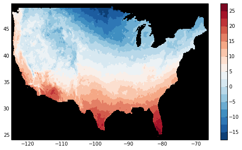
Now, let’s access and plot a small subset:
In [99]: tmax_ss = tmax[0]
For this dataset, we still need to manually fill in some of the values with NaN to indicate that they are missing. As soon as we access tmax_ss.values, the values are loaded over the network and cached on the DataArray so they can be manipulated:
In [100]: tmax_ss.values[tmax_ss.values < -99] = np.nan
Finally, we can plot the values with matplotlib:
In [101]: import matplotlib.pyplot as plt

In [102]: from matplotlib.cm import get_cmap

In [103]: plt.figure(figsize=(9, 5))

In [104]: plt.gca().patch.set_color('0')

In [105]: plt.contourf(tmax_ss['X'], tmax_ss['Y'], tmax_ss.values, 20,
             cmap=get_cmap('RdBu_r'))

In [106]: plt.colorbar()