Reading and writing files

Xarray supports direct serialization and IO to several file formats, from simple Pickle files to the more flexible netCDF format (recommended).

You can read different types of files in xr.open_dataset by specifying the engine to be used:

xr.open_dataset("example.nc", engine="netcdf4")

The “engine” provides a set of instructions that tells xarray how to read the data and pack them into a Dataset (or Dataarray). These instructions are stored in an underlying “backend”.

Xarray comes with several backends that cover many common data formats. Many more backends are available via external libraries, or you can write your own. This diagram aims to help you determine - based on the format of the file you’d like to read - which type of backend you’re using and how to use it.

Text and boxes are clickable for more information. Following the diagram is detailed information on many popular backends. You can learn more about using and developing backends in the Xarray tutorial JupyterBook.

        flowchart LR
    built-in-eng["""Is your data stored in one of these formats?
        - netCDF4 (<code>netcdf4</code>)
        - netCDF3 (<code>scipy</code>)
        - Zarr (<code>zarr</code>)
        - DODS/OPeNDAP (<code>pydap</code>)
        - HDF5 (<code>h5netcdf</code>)
        """]

    built-in("""You're in luck! Xarray bundles a backend for this format.
        Open data using <code>xr.open_dataset()</code>. We recommend
        always setting the engine you want to use.""")

    installed-eng["""One of these formats?
        - <a href='https://github.com/ecmwf/cfgrib'>GRIB (<code>cfgrib</code>)
        - <a href='https://tiledb-inc.github.io/TileDB-CF-Py/documentation/index.html'>TileDB (<code>tiledb</code>)
        - <a href='https://corteva.github.io/rioxarray/stable/getting_started/getting_started.html#rioxarray'>GeoTIFF, JPEG-2000, ESRI-hdf (<code>rioxarray</code>, via GDAL)
        - <a href='https://www.bopen.eu/xarray-sentinel-open-source-library/'>Sentinel-1 SAFE (<code>xarray-sentinel</code>)
        """]

    installed("""Install the package indicated in parentheses to your
        Python environment. Restart the kernel and use
        <code>xr.open_dataset(files, engine='rioxarray')</code>.""")

    other("""Ask around to see if someone in your data community
        has created an Xarray backend for your data type.
        If not, you may need to create your own or consider
        exporting your data to a more common format.""")

    built-in-eng -->|Yes| built-in
    built-in-eng -->|No| installed-eng

    installed-eng -->|Yes| installed
    installed-eng -->|No| other

    click built-in-eng "https://docs.xarray.dev/en/stable/getting-started-guide/faq.html#how-do-i-open-format-x-file-as-an-xarray-dataset"
    click other "https://docs.xarray.dev/en/stable/internals/how-to-add-new-backend.html"

    classDef quesNodefmt fill:#9DEEF4,stroke:#206C89,text-align:left
    class built-in-eng,installed-eng quesNodefmt

    classDef ansNodefmt fill:#FFAA05,stroke:#E37F17,text-align:left,white-space:nowrap
    class built-in,installed,other ansNodefmt

    linkStyle default font-size:20pt,color:#206C89
    

netCDF

The recommended way to store xarray data structures is netCDF, which is a binary file format for self-described datasets that originated in the geosciences. Xarray is based on the netCDF data model, so netCDF files on disk directly correspond to Dataset objects (more accurately, a group in a netCDF file directly corresponds to a Dataset object. See Groups for more.)

NetCDF is supported on almost all platforms, and parsers exist for the vast majority of scientific programming languages. Recent versions of netCDF are based on the even more widely used HDF5 file-format.

Tip

If you aren’t familiar with this data format, the netCDF FAQ is a good place to start.

Reading and writing netCDF files with xarray requires scipy, h5netcdf, or the netCDF4-Python library to be installed. SciPy only supports reading and writing of netCDF V3 files.

We can save a Dataset to disk using the Dataset.to_netcdf() method:

In [1]: ds = xr.Dataset(
   ...:     {"foo": (("x", "y"), np.random.rand(4, 5))},
   ...:     coords={
   ...:         "x": [10, 20, 30, 40],
   ...:         "y": pd.date_range("2000-01-01", periods=5),
   ...:         "z": ("x", list("abcd")),
   ...:     },
   ...: )
   ...: 

In [2]: ds.to_netcdf("saved_on_disk.nc")

By default, the file is saved as netCDF4 (assuming netCDF4-Python is installed). You can control the format and engine used to write the file with the format and engine arguments.

Tip

Using the h5netcdf package by passing engine='h5netcdf' to open_dataset() can sometimes be quicker than the default engine='netcdf4' that uses the netCDF4 package.

We can load netCDF files to create a new Dataset using open_dataset():

In [3]: ds_disk = xr.open_dataset("saved_on_disk.nc")

In [4]: ds_disk
Out[4]: 
<xarray.Dataset> Size: 248B
Dimensions:  (x: 4, y: 5)
Coordinates:
  * x        (x) int64 32B 10 20 30 40
  * y        (y) datetime64[ns] 40B 2000-01-01 2000-01-02 ... 2000-01-05
    z        (x) <U1 16B ...
Data variables:
    foo      (x, y) float64 160B ...

Similarly, a DataArray can be saved to disk using the DataArray.to_netcdf() method, and loaded from disk using the open_dataarray() function. As netCDF files correspond to Dataset objects, these functions internally convert the DataArray to a Dataset before saving, and then convert back when loading, ensuring that the DataArray that is loaded is always exactly the same as the one that was saved.

A dataset can also be loaded or written to a specific group within a netCDF file. To load from a group, pass a group keyword argument to the open_dataset function. The group can be specified as a path-like string, e.g., to access subgroup ‘bar’ within group ‘foo’ pass ‘/foo/bar’ as the group argument. When writing multiple groups in one file, pass mode='a' to to_netcdf to ensure that each call does not delete the file.

Tip

It is recommended to use DataTree to represent hierarchical data, and to use the xarray.DataTree.to_netcdf() method when writing hierarchical data to a netCDF file.

Data is always loaded lazily from netCDF files. You can manipulate, slice and subset Dataset and DataArray objects, and no array values are loaded into memory until you try to perform some sort of actual computation. For an example of how these lazy arrays work, see the OPeNDAP section below.

There may be minor differences in the Dataset object returned when reading a NetCDF file with different engines.

It is important to note that when you modify values of a Dataset, even one linked to files on disk, only the in-memory copy you are manipulating in xarray is modified: the original file on disk is never touched.

Tip

Xarray’s lazy loading of remote or on-disk datasets is often but not always desirable. Before performing computationally intense operations, it is often a good idea to load a Dataset (or DataArray) entirely into memory by invoking the Dataset.load() method.

Datasets have a Dataset.close() method to close the associated netCDF file. However, it’s often cleaner to use a with statement:

# this automatically closes the dataset after use
In [5]: with xr.open_dataset("saved_on_disk.nc") as ds:
   ...:     print(ds.keys())
   ...: 
KeysView(<xarray.Dataset> Size: 248B
Dimensions:  (x: 4, y: 5)
Coordinates:
  * x        (x) int64 32B 10 20 30 40
  * y        (y) datetime64[ns] 40B 2000-01-01 2000-01-02 ... 2000-01-05
    z        (x) <U1 16B ...
Data variables:
    foo      (x, y) float64 160B ...)

Although xarray provides reasonable support for incremental reads of files on disk, it does not support incremental writes, which can be a useful strategy for dealing with datasets too big to fit into memory. Instead, xarray integrates with dask.array (see Parallel Computing with Dask), which provides a fully featured engine for streaming computation.

It is possible to append or overwrite netCDF variables using the mode='a' argument. When using this option, all variables in the dataset will be written to the original netCDF file, regardless if they exist in the original dataset.

Groups

Whilst netCDF groups can only be loaded individually as Dataset objects, a whole file of many nested groups can be loaded as a single xarray.DataTree object. To open a whole netCDF file as a tree of groups use the xarray.open_datatree() function. To save a DataTree object as a netCDF file containing many groups, use the xarray.DataTree.to_netcdf() method.

Note

Due to file format specifications the on-disk root group name is always "/", overriding any given DataTree root node name.

Warning

DataTree objects do not follow the exact same data model as netCDF files, which means that perfect round-tripping is not always possible.

In particular in the netCDF data model dimensions are entities that can exist regardless of whether any variable possesses them. This is in contrast to xarray’s data model (and hence DataTree’s data model) in which the dimensions of a (Dataset/Tree) object are simply the set of dimensions present across all variables in that dataset.

This means that if a netCDF file contains dimensions but no variables which possess those dimensions, these dimensions will not be present when that file is opened as a DataTree object. Saving this DataTree object to file will therefore not preserve these “unused” dimensions.

Reading encoded data

NetCDF files follow some conventions for encoding datetime arrays (as numbers with a “units” attribute) and for packing and unpacking data (as described by the “scale_factor” and “add_offset” attributes). If the argument decode_cf=True (default) is given to open_dataset(), xarray will attempt to automatically decode the values in the netCDF objects according to CF conventions. Sometimes this will fail, for example, if a variable has an invalid “units” or “calendar” attribute. For these cases, you can turn this decoding off manually.

You can view this encoding information (among others) in the DataArray.encoding and DataArray.encoding attributes:

In [6]: ds_disk["y"].encoding
Out[6]: 
{'dtype': dtype('int64'),
 'zlib': False,
 'szip': False,
 'zstd': False,
 'bzip2': False,
 'blosc': False,
 'shuffle': False,
 'complevel': 0,
 'fletcher32': False,
 'contiguous': True,
 'chunksizes': None,
 'source': '/home/docs/checkouts/readthedocs.org/user_builds/xray/checkouts/latest/doc/saved_on_disk.nc',
 'original_shape': (5,),
 'units': 'days since 2000-01-01 00:00:00',
 'calendar': 'proleptic_gregorian'}

In [7]: ds_disk.encoding
Out[7]: 
{'unlimited_dims': set(),
 'source': '/home/docs/checkouts/readthedocs.org/user_builds/xray/checkouts/latest/doc/saved_on_disk.nc'}

Note that all operations that manipulate variables other than indexing will remove encoding information.

In some cases it is useful to intentionally reset a dataset’s original encoding values. This can be done with either the Dataset.drop_encoding() or DataArray.drop_encoding() methods.

In [8]: ds_no_encoding = ds_disk.drop_encoding()

In [9]: ds_no_encoding.encoding
Out[9]: {}

Reading multi-file datasets

NetCDF files are often encountered in collections, e.g., with different files corresponding to different model runs or one file per timestamp. Xarray can straightforwardly combine such files into a single Dataset by making use of concat(), merge(), combine_nested() and combine_by_coords(). For details on the difference between these functions see Combining data.

Xarray includes support for manipulating datasets that don’t fit into memory with dask. If you have dask installed, you can open multiple files simultaneously in parallel using open_mfdataset():

xr.open_mfdataset('my/files/*.nc', parallel=True)

This function automatically concatenates and merges multiple files into a single xarray dataset. It is the recommended way to open multiple files with xarray. For more details on parallel reading, see Combining along multiple dimensions, Reading and writing data and a blog post by Stephan Hoyer. open_mfdataset() takes many kwargs that allow you to control its behaviour (for e.g. parallel, combine, compat, join, concat_dim). See its docstring for more details.

Note

A common use-case involves a dataset distributed across a large number of files with each file containing a large number of variables. Commonly, a few of these variables need to be concatenated along a dimension (say "time"), while the rest are equal across the datasets (ignoring floating point differences). The following command with suitable modifications (such as parallel=True) works well with such datasets:

xr.open_mfdataset('my/files/*.nc', concat_dim="time", combine="nested",
                  data_vars='minimal', coords='minimal', compat='override')

This command concatenates variables along the "time" dimension, but only those that already contain the "time" dimension (data_vars='minimal', coords='minimal'). Variables that lack the "time" dimension are taken from the first dataset (compat='override').

Sometimes multi-file datasets are not conveniently organized for easy use of open_mfdataset(). One can use the preprocess argument to provide a function that takes a dataset and returns a modified Dataset. open_mfdataset() will call preprocess on every dataset (corresponding to each file) prior to combining them.

If open_mfdataset() does not meet your needs, other approaches are possible. The general pattern for parallel reading of multiple files using dask, modifying those datasets and then combining into a single Dataset is:

def modify(ds):
    # modify ds here
    return ds


# this is basically what open_mfdataset does
open_kwargs = dict(decode_cf=True, decode_times=False)
open_tasks = [dask.delayed(xr.open_dataset)(f, **open_kwargs) for f in file_names]
tasks = [dask.delayed(modify)(task) for task in open_tasks]
datasets = dask.compute(tasks)  # get a list of xarray.Datasets
combined = xr.combine_nested(datasets)  # or some combination of concat, merge

As an example, here’s how we could approximate MFDataset from the netCDF4 library:

from glob import glob
import xarray as xr

def read_netcdfs(files, dim):
    # glob expands paths with * to a list of files, like the unix shell
    paths = sorted(glob(files))
    datasets = [xr.open_dataset(p) for p in paths]
    combined = xr.concat(datasets, dim)
    return combined

combined = read_netcdfs('/all/my/files/*.nc', dim='time')

This function will work in many cases, but it’s not very robust. First, it never closes files, which means it will fail if you need to load more than a few thousand files. Second, it assumes that you want all the data from each file and that it can all fit into memory. In many situations, you only need a small subset or an aggregated summary of the data from each file.

Here’s a slightly more sophisticated example of how to remedy these deficiencies:

def read_netcdfs(files, dim, transform_func=None):
    def process_one_path(path):
        # use a context manager, to ensure the file gets closed after use
        with xr.open_dataset(path) as ds:
            # transform_func should do some sort of selection or
            # aggregation
            if transform_func is not None:
                ds = transform_func(ds)
            # load all data from the transformed dataset, to ensure we can
            # use it after closing each original file
            ds.load()
            return ds

    paths = sorted(glob(files))
    datasets = [process_one_path(p) for p in paths]
    combined = xr.concat(datasets, dim)
    return combined

# here we suppose we only care about the combined mean of each file;
# you might also use indexing operations like .sel to subset datasets
combined = read_netcdfs('/all/my/files/*.nc', dim='time',
                        transform_func=lambda ds: ds.mean())

This pattern works well and is very robust. We’ve used similar code to process tens of thousands of files constituting 100s of GB of data.

Writing encoded data

Conversely, you can customize how xarray writes netCDF files on disk by providing explicit encodings for each dataset variable. The encoding argument takes a dictionary with variable names as keys and variable specific encodings as values. These encodings are saved as attributes on the netCDF variables on disk, which allows xarray to faithfully read encoded data back into memory.

It is important to note that using encodings is entirely optional: if you do not supply any of these encoding options, xarray will write data to disk using a default encoding, or the options in the encoding attribute, if set. This works perfectly fine in most cases, but encoding can be useful for additional control, especially for enabling compression.

In the file on disk, these encodings are saved as attributes on each variable, which allow xarray and other CF-compliant tools for working with netCDF files to correctly read the data.

Scaling and type conversions

These encoding options (based on CF Conventions on packed data) work on any version of the netCDF file format:

• dtype: Any valid NumPy dtype or string convertible to a dtype, e.g., 'int16' or 'float32'. This controls the type of the data written on disk.

• _FillValue: Values of NaN in xarray variables are remapped to this value when saved on disk. This is important when converting floating point with missing values to integers on disk, because NaN is not a valid value for integer dtypes. By default, variables with float types are attributed a _FillValue of NaN in the output file, unless explicitly disabled with an encoding {'_FillValue': None}.

• scale_factor and add_offset: Used to convert from encoded data on disk to to the decoded data in memory, according to the formula decoded = scale_factor * encoded + add_offset. Please note that scale_factor and add_offset must be of same type and determine the type of the decoded data.

These parameters can be fruitfully combined to compress discretized data on disk. For example, to save the variable foo with a precision of 0.1 in 16-bit integers while converting NaN to -9999, we would use encoding={'foo': {'dtype': 'int16', 'scale_factor': 0.1, '_FillValue': -9999}}. Compression and decompression with such discretization is extremely fast.

String encoding

Xarray can write unicode strings to netCDF files in two ways:

• As variable length strings. This is only supported on netCDF4 (HDF5) files.

• By encoding strings into bytes, and writing encoded bytes as a character array. The default encoding is UTF-8.

By default, we use variable length strings for compatible files and fall-back to using encoded character arrays. Character arrays can be selected even for netCDF4 files by setting the dtype field in encoding to S1 (corresponding to NumPy’s single-character bytes dtype).

If character arrays are used:

• The string encoding that was used is stored on disk in the _Encoding attribute, which matches an ad-hoc convention adopted by the netCDF4-Python library. At the time of this writing (October 2017), a standard convention for indicating string encoding for character arrays in netCDF files was still under discussion. Technically, you can use any string encoding recognized by Python if you feel the need to deviate from UTF-8, by setting the _Encoding field in encoding. But we don’t recommend it.

• The character dimension name can be specified by the char_dim_name field of a variable’s encoding. If the name of the character dimension is not specified, the default is f'string{data.shape[-1]}'. When decoding character arrays from existing files, the char_dim_name is added to the variables encoding to preserve if encoding happens, but the field can be edited by the user.

Warning

Missing values in bytes or unicode string arrays (represented by NaN in xarray) are currently written to disk as empty strings ''. This means missing values will not be restored when data is loaded from disk. This behavior is likely to change in the future (GH1647). Unfortunately, explicitly setting a _FillValue for string arrays to handle missing values doesn’t work yet either, though we also hope to fix this in the future.

Chunk based compression

zlib, complevel, fletcher32, contiguous and chunksizes can be used for enabling netCDF4/HDF5’s chunk based compression, as described in the documentation for createVariable for netCDF4-Python. This only works for netCDF4 files and thus requires using format='netCDF4' and either engine='netcdf4' or engine='h5netcdf'.

Chunk based gzip compression can yield impressive space savings, especially for sparse data, but it comes with significant performance overhead. HDF5 libraries can only read complete chunks back into memory, and maximum decompression speed is in the range of 50-100 MB/s. Worse, HDF5’s compression and decompression currently cannot be parallelized with dask. For these reasons, we recommend trying discretization based compression (described above) first.

Time units

The units and calendar attributes control how xarray serializes datetime64 and timedelta64 arrays to datasets on disk as numeric values. The units encoding should be a string like 'days since 1900-01-01' for datetime64 data or a string like 'days' for timedelta64 data. calendar should be one of the calendar types supported by netCDF4-python: ‘standard’, ‘gregorian’, ‘proleptic_gregorian’ ‘noleap’, ‘365_day’, ‘360_day’, ‘julian’, ‘all_leap’, ‘366_day’.

By default, xarray uses the 'proleptic_gregorian' calendar and units of the smallest time difference between values, with a reference time of the first time value.

Coordinates

You can control the coordinates attribute written to disk by specifying DataArray.encoding["coordinates"]. If not specified, xarray automatically sets DataArray.encoding["coordinates"] to a space-delimited list of names of coordinate variables that share dimensions with the DataArray being written. This allows perfect roundtripping of xarray datasets but may not be desirable. When an xarray Dataset contains non-dimensional coordinates that do not share dimensions with any of the variables, these coordinate variable names are saved under a “global” "coordinates" attribute. This is not CF-compliant but again facilitates roundtripping of xarray datasets.

Invalid netCDF files

The library h5netcdf allows writing some dtypes that aren’t allowed in netCDF4 (see h5netcdf documentation). This feature is available through DataArray.to_netcdf() and Dataset.to_netcdf() when used with engine="h5netcdf" and currently raises a warning unless invalid_netcdf=True is set.

Warning

Note that this produces a file that is likely to be not readable by other netCDF libraries!

HDF5

HDF5 is both a file format and a data model for storing information. HDF5 stores data hierarchically, using groups to create a nested structure. HDF5 is a more general version of the netCDF4 data model, so the nested structure is one of many similarities between the two data formats.

Reading HDF5 files in xarray requires the h5netcdf engine, which can be installed with conda install h5netcdf. Once installed we can use xarray to open HDF5 files:

xr.open_dataset("/path/to/my/file.h5")

The similarities between HDF5 and netCDF4 mean that HDF5 data can be written with the same Dataset.to_netcdf() method as used for netCDF4 data:

In [10]: ds = xr.Dataset(
   ....:     {"foo": (("x", "y"), np.random.rand(4, 5))},
   ....:     coords={
   ....:         "x": [10, 20, 30, 40],
   ....:         "y": pd.date_range("2000-01-01", periods=5),
   ....:         "z": ("x", list("abcd")),
   ....:     },
   ....: )
   ....: 

In [11]: ds.to_netcdf("saved_on_disk.h5")

Groups

If you have multiple or highly nested groups, xarray by default may not read the group that you want. A particular group of an HDF5 file can be specified using the group argument:

xr.open_dataset("/path/to/my/file.h5", group="/my/group")

While xarray cannot interrogate an HDF5 file to determine which groups are available, the HDF5 Python reader h5py can be used instead.

Natively the xarray data structures can only handle one level of nesting, organized as DataArrays inside of Datasets. If your HDF5 file has additional levels of hierarchy you can only access one group and a time and will need to specify group names.

Zarr

Zarr is a Python package that provides an implementation of chunked, compressed, N-dimensional arrays. Zarr has the ability to store arrays in a range of ways, including in memory, in files, and in cloud-based object storage such as Amazon S3 and Google Cloud Storage. Xarray’s Zarr backend allows xarray to leverage these capabilities, including the ability to store and analyze datasets far too large fit onto disk (particularly in combination with dask).

Xarray can’t open just any zarr dataset, because xarray requires special metadata (attributes) describing the dataset dimensions and coordinates. At this time, xarray can only open zarr datasets with these special attributes, such as zarr datasets written by xarray, netCDF, or GDAL. For implementation details, see Zarr Encoding Specification.

To write a dataset with zarr, we use the Dataset.to_zarr() method.

To write to a local directory, we pass a path to a directory:

In [12]: ds = xr.Dataset(
   ....:     {"foo": (("x", "y"), np.random.rand(4, 5))},
   ....:     coords={
   ....:         "x": [10, 20, 30, 40],
   ....:         "y": pd.date_range("2000-01-01", periods=5),
   ....:         "z": ("x", list("abcd")),
   ....:     },
   ....: )
   ....: 

In [13]: ds.to_zarr("path/to/directory.zarr")
Out[13]: <xarray.backends.zarr.ZarrStore at 0x7fa385cec550>

(The suffix .zarr is optional–just a reminder that a zarr store lives there.) If the directory does not exist, it will be created. If a zarr store is already present at that path, an error will be raised, preventing it from being overwritten. To override this behavior and overwrite an existing store, add mode='w' when invoking to_zarr().

DataArrays can also be saved to disk using the DataArray.to_zarr() method, and loaded from disk using the open_dataarray() function with engine='zarr'. Similar to DataArray.to_netcdf(), DataArray.to_zarr() will convert the DataArray to a Dataset before saving, and then convert back when loading, ensuring that the DataArray that is loaded is always exactly the same as the one that was saved.

Note

xarray does not write NCZarr attributes. Therefore, NCZarr data must be opened in read-only mode.

To store variable length strings, convert them to object arrays first with dtype=object.

To read back a zarr dataset that has been created this way, we use the open_zarr() method:

In [14]: ds_zarr = xr.open_zarr("path/to/directory.zarr")

In [15]: ds_zarr
Out[15]: 
<xarray.Dataset> Size: 264B
Dimensions:  (x: 4, y: 5)
Coordinates:
    z        (x) object 32B dask.array<chunksize=(4,), meta=np.ndarray>
  * y        (y) datetime64[ns] 40B 2000-01-01 2000-01-02 ... 2000-01-05
  * x        (x) int64 32B 10 20 30 40
Data variables:
    foo      (x, y) float64 160B dask.array<chunksize=(4, 5), meta=np.ndarray>

Cloud Storage Buckets

It is possible to read and write xarray datasets directly from / to cloud storage buckets using zarr. This example uses the gcsfs package to provide an interface to Google Cloud Storage.

General fsspec URLs, those that begin with s3:// or gcs:// for example, are parsed and the store set up for you automatically when reading. You should include any arguments to the storage backend as the key `storage_options, part of backend_kwargs.

ds_gcs = xr.open_dataset(
    "gcs://<bucket-name>/path.zarr",
    backend_kwargs={
        "storage_options": {"project": "<project-name>", "token": None}
    },
    engine="zarr",
)

This also works with open_mfdataset, allowing you to pass a list of paths or a URL to be interpreted as a glob string.

For writing, you must explicitly set up a MutableMapping instance and pass this, as follows:

import gcsfs

fs = gcsfs.GCSFileSystem(project="<project-name>", token=None)
gcsmap = gcsfs.mapping.GCSMap("<bucket-name>", gcs=fs, check=True, create=False)
# write to the bucket
ds.to_zarr(store=gcsmap)
# read it back
ds_gcs = xr.open_zarr(gcsmap)

(or use the utility function fsspec.get_mapper()).

Distributed writes

Xarray will natively use dask to write in parallel to a zarr store, which should satisfy most moderately sized datasets. For more flexible parallelization, we can use region to write to limited regions of arrays in an existing Zarr store.

To scale this up to writing large datasets, first create an initial Zarr store without writing all of its array data. This can be done by first creating a Dataset with dummy values stored in dask, and then calling to_zarr with compute=False to write only metadata (including attrs) to Zarr:

In [16]: import dask.array

# The values of this dask array are entirely irrelevant; only the dtype,
# shape and chunks are used
In [17]: dummies = dask.array.zeros(30, chunks=10)

In [18]: ds = xr.Dataset({"foo": ("x", dummies)}, coords={"x": np.arange(30)})

In [19]: path = "path/to/directory.zarr"

# Now we write the metadata without computing any array values
In [20]: ds.to_zarr(path, compute=False)
Out[20]: Delayed('_finalize_store-dd0aa610-c51b-42c6-b6f1-4c54c5724487')

Now, a Zarr store with the correct variable shapes and attributes exists that can be filled out by subsequent calls to to_zarr. Setting region="auto" will open the existing store and determine the correct alignment of the new data with the existing dimensions, or as an explicit mapping from dimension names to Python slice objects indicating where the data should be written (in index space, not label space), e.g.,

# For convenience, we'll slice a single dataset, but in the real use-case
# we would create them separately possibly even from separate processes.
In [21]: ds = xr.Dataset({"foo": ("x", np.arange(30))}, coords={"x": np.arange(30)})

# Any of the following region specifications are valid
In [22]: ds.isel(x=slice(0, 10)).to_zarr(path, region="auto")
Out[22]: <xarray.backends.zarr.ZarrStore at 0x7fa385f6f130>

In [23]: ds.isel(x=slice(10, 20)).to_zarr(path, region={"x": "auto"})
Out[23]: <xarray.backends.zarr.ZarrStore at 0x7fa385cee5f0>

In [24]: ds.isel(x=slice(20, 30)).to_zarr(path, region={"x": slice(20, 30)})
Out[24]: <xarray.backends.zarr.ZarrStore at 0x7fa387154ca0>

Concurrent writes with region are safe as long as they modify distinct chunks in the underlying Zarr arrays (or use an appropriate lock).

As a safety check to make it harder to inadvertently override existing values, if you set region then all variables included in a Dataset must have dimensions included in region. Other variables (typically coordinates) need to be explicitly dropped and/or written in a separate calls to to_zarr with mode='a'.

Zarr Compressors and Filters

There are many different options for compression and filtering possible with zarr.

These options can be passed to the to_zarr method as variable encoding. For example:

In [25]: import zarr

In [26]: from numcodecs.blosc import Blosc

In [27]: compressor = Blosc(cname="zstd", clevel=3, shuffle=2)

In [28]: ds.to_zarr("foo.zarr", encoding={"foo": {"compressor": compressor}})
TypeError: Expected a BytesBytesCodec. Got <class 'numcodecs.blosc.Blosc'> instead.

Note

Not all native zarr compression and filtering options have been tested with xarray.

Modifying existing Zarr stores

Xarray supports several ways of incrementally writing variables to a Zarr store. These options are useful for scenarios when it is infeasible or undesirable to write your entire dataset at once.

1. Use mode='a' to add or overwrite entire variables,

2. Use append_dim to resize and append to existing variables, and

3. Use region to write to limited regions of existing arrays.

Tip

For Dataset objects containing dask arrays, a single call to to_zarr() will write all of your data in parallel.

Warning

Alignment of coordinates is currently not checked when modifying an existing Zarr store. It is up to the user to ensure that coordinates are consistent.

To add or overwrite entire variables, simply call to_zarr() with mode='a' on a Dataset containing the new variables, passing in an existing Zarr store or path to a Zarr store.

To resize and then append values along an existing dimension in a store, set append_dim. This is a good option if data always arrives in a particular order, e.g., for time-stepping a simulation:

In [29]: ds1 = xr.Dataset(
   ....:     {"foo": (("x", "y", "t"), np.random.rand(4, 5, 2))},
   ....:     coords={
   ....:         "x": [10, 20, 30, 40],
   ....:         "y": [1, 2, 3, 4, 5],
   ....:         "t": pd.date_range("2001-01-01", periods=2),
   ....:     },
   ....: )
   ....: 

In [30]: ds1.to_zarr("path/to/directory.zarr")
Out[30]: <xarray.backends.zarr.ZarrStore at 0x7fa385f6e200>

In [31]: ds2 = xr.Dataset(
   ....:     {"foo": (("x", "y", "t"), np.random.rand(4, 5, 2))},
   ....:     coords={
   ....:         "x": [10, 20, 30, 40],
   ....:         "y": [1, 2, 3, 4, 5],
   ....:         "t": pd.date_range("2001-01-03", periods=2),
   ....:     },
   ....: )
   ....: 

In [32]: ds2.to_zarr("path/to/directory.zarr", append_dim="t")
Out[32]: <xarray.backends.zarr.ZarrStore at 0x7fa385ceef80>

Specifying chunks in a zarr store

Chunk sizes may be specified in one of three ways when writing to a zarr store:

1. Manual chunk sizing through the use of the encoding argument in Dataset.to_zarr():

2. Automatic chunking based on chunks in dask arrays

3. Default chunk behavior determined by the zarr library

The resulting chunks will be determined based on the order of the above list; dask chunks will be overridden by manually-specified chunks in the encoding argument, and the presence of either dask chunks or chunks in the encoding attribute will supersede the default chunking heuristics in zarr.

Importantly, this logic applies to every array in the zarr store individually, including coordinate arrays. Therefore, if a dataset contains one or more dask arrays, it may still be desirable to specify a chunk size for the coordinate arrays (for example, with a chunk size of -1 to include the full coordinate).

To specify chunks manually using the encoding argument, provide a nested dictionary with the structure {'variable_or_coord_name': {'chunks': chunks_tuple}}.

Note

The positional ordering of the chunks in the encoding argument must match the positional ordering of the dimensions in each array. Watch out for arrays with differently-ordered dimensions within a single Dataset.

For example, let’s say we’re working with a dataset with dimensions ('time', 'x', 'y'), a variable Tair which is chunked in x and y, and two multi-dimensional coordinates xc and yc:

In [33]: ds = xr.tutorial.open_dataset("rasm")

In [34]: ds["Tair"] = ds["Tair"].chunk({"x": 100, "y": 100})

In [35]: ds
Out[35]: 
<xarray.Dataset> Size: 17MB
Dimensions:  (time: 36, y: 205, x: 275)
Coordinates:
  * time     (time) object 288B 1980-09-16 12:00:00 ... 1983-08-17 00:00:00
    xc       (y, x) float64 451kB ...
    yc       (y, x) float64 451kB ...
Dimensions without coordinates: y, x
Data variables:
    Tair     (time, y, x) float64 16MB dask.array<chunksize=(36, 100, 100), meta=np.ndarray>
Attributes:
    title:                     /workspace/jhamman/processed/R1002RBRxaaa01a/l...
    institution:               U.W.
    source:                    RACM R1002RBRxaaa01a
    output_frequency:          daily
    output_mode:               averaged
    convention:                CF-1.4
    references:                Based on the initial model of Liang et al., 19...
    comment:                   Output from the Variable Infiltration Capacity...
    nco_openmp_thread_number:  1
    NCO:                       netCDF Operators version 4.7.9 (Homepage = htt...
    history:                   Fri Aug  7 17:57:38 2020: ncatted -a bounds,,d...

These multi-dimensional coordinates are only two-dimensional and take up very little space on disk or in memory, yet when writing to disk the default zarr behavior is to split them into chunks:

In [36]: ds.to_zarr("path/to/directory.zarr", mode="w")
Out[36]: <xarray.backends.zarr.ZarrStore at 0x7fa385cef7f0>

In [37]: ! ls -R path/to/directory.zarr
path/to/directory.zarr:
Tair  foo  t  time  x  xc  y  yc  zarr.json

path/to/directory.zarr/Tair:
c  zarr.json

path/to/directory.zarr/Tair/c:
0

path/to/directory.zarr/Tair/c/0:
0  1  2

path/to/directory.zarr/Tair/c/0/0:
0  1  2

path/to/directory.zarr/Tair/c/0/1:
0  1  2

path/to/directory.zarr/Tair/c/0/2:
0  1  2

path/to/directory.zarr/foo:
c

path/to/directory.zarr/foo/c:
0

path/to/directory.zarr/foo/c/0:
0

path/to/directory.zarr/foo/c/0/0:

path/to/directory.zarr/t:
c

path/to/directory.zarr/t/c:

path/to/directory.zarr/time:
c  zarr.json

path/to/directory.zarr/time/c:
0

path/to/directory.zarr/x:
c

path/to/directory.zarr/x/c:

path/to/directory.zarr/xc:
c  zarr.json

path/to/directory.zarr/xc/c:
0  1

path/to/directory.zarr/xc/c/0:
0

path/to/directory.zarr/xc/c/1:
0

path/to/directory.zarr/y:
c

path/to/directory.zarr/y/c:

path/to/directory.zarr/yc:
c  zarr.json

path/to/directory.zarr/yc/c:
0  1

path/to/directory.zarr/yc/c/0:
0

path/to/directory.zarr/yc/c/1:
0

This may cause unwanted overhead on some systems, such as when reading from a cloud storage provider. To disable this chunking, we can specify a chunk size equal to the length of each dimension by using the shorthand chunk size -1:

In [38]: ds.to_zarr(
   ....:     "path/to/directory.zarr",
   ....:     encoding={"xc": {"chunks": (-1, -1)}, "yc": {"chunks": (-1, -1)}},
   ....:     mode="w",
   ....: )
   ....: 
ValueError: Expected all values to be non-negative. Got (-1, -1) instead.


In [39]: ! ls -R path/to/directory.zarr
path/to/directory.zarr:
Tair  foo  t  time  x  xc  y  yc  zarr.json

path/to/directory.zarr/Tair:
c

path/to/directory.zarr/Tair/c:
0

path/to/directory.zarr/Tair/c/0:
0  1  2

path/to/directory.zarr/Tair/c/0/0:

path/to/directory.zarr/Tair/c/0/1:

path/to/directory.zarr/Tair/c/0/2:

path/to/directory.zarr/foo:
c

path/to/directory.zarr/foo/c:
0

path/to/directory.zarr/foo/c/0:
0

path/to/directory.zarr/foo/c/0/0:

path/to/directory.zarr/t:
c

path/to/directory.zarr/t/c:

path/to/directory.zarr/time:
c  zarr.json

path/to/directory.zarr/time/c:
0

path/to/directory.zarr/x:
c

path/to/directory.zarr/x/c:

path/to/directory.zarr/xc:
c

path/to/directory.zarr/xc/c:
0  1

path/to/directory.zarr/xc/c/0:

path/to/directory.zarr/xc/c/1:

path/to/directory.zarr/y:
c

path/to/directory.zarr/y/c:

path/to/directory.zarr/yc:
c

path/to/directory.zarr/yc/c:
0  1

path/to/directory.zarr/yc/c/0:

path/to/directory.zarr/yc/c/1:

The number of chunks on Tair matches our dask chunks, while there is now only a single chunk in the directory stores of each coordinate.

Groups

Nested groups in zarr stores can be represented by loading the store as a xarray.DataTree object, similarly to netCDF. To open a whole zarr store as a tree of groups use the open_datatree() function. To save a DataTree object as a zarr store containing many groups, use the xarray.DataTree.to_zarr() method.

Note

Note that perfect round-tripping should always be possible with a zarr store (unlike for netCDF files), as zarr does not support “unused” dimensions.

For the root group the same restrictions (as for netCDF files) apply. Due to file format specifications the on-disk root group name is always "/" overriding any given DataTree root node name.

Consolidated Metadata

Xarray needs to read all of the zarr metadata when it opens a dataset. In some storage mediums, such as with cloud object storage (e.g. Amazon S3), this can introduce significant overhead, because two separate HTTP calls to the object store must be made for each variable in the dataset. By default Xarray uses a feature called consolidated metadata, storing all metadata for the entire dataset with a single key (by default called .zmetadata). This typically drastically speeds up opening the store. (For more information on this feature, consult the zarr docs on consolidating metadata.)

By default, xarray writes consolidated metadata and attempts to read stores with consolidated metadata, falling back to use non-consolidated metadata for reads. Because this fall-back option is so much slower, xarray issues a RuntimeWarning with guidance when reading with consolidated metadata fails:

Failed to open Zarr store with consolidated metadata, falling back to try reading non-consolidated metadata. This is typically much slower for opening a dataset. To silence this warning, consider:

1. Consolidating metadata in this existing store with zarr.consolidate_metadata().

2. Explicitly setting consolidated=False, to avoid trying to read consolidate metadata.

3. Explicitly setting consolidated=True, to raise an error in this case instead of falling back to try reading non-consolidated metadata.

Kerchunk

Kerchunk is a Python library that allows you to access chunked and compressed data formats (such as NetCDF3, NetCDF4, HDF5, GRIB2, TIFF & FITS), many of which are primary data formats for many data archives, by viewing the whole archive as an ephemeral Zarr dataset which allows for parallel, chunk-specific access.

Instead of creating a new copy of the dataset in the Zarr spec/format or downloading the files locally, Kerchunk reads through the data archive and extracts the byte range and compression information of each chunk and saves as a reference. These references are then saved as json files or parquet (more efficient) for later use. You can view some of these stored in the references directory here.

Note

These references follow this specification. Packages like kerchunk and virtualizarr help in creating and reading these references.

Reading these data archives becomes really easy with kerchunk in combination with xarray, especially when these archives are large in size. A single combined reference can refer to thousands of the original data files present in these archives. You can view the whole dataset with from this combined reference using the above packages.

The following example shows opening a combined references generated from a .hdf file stored locally.

In [40]: storage_options = {
   ....:     "target_protocol": "file",
   ....: }
   ....: 

# add the `remote_protocol` key in `storage_options` if you're accessing a file remotely
In [41]: ds1 = xr.open_dataset(
   ....:     "./combined.json",
   ....:     engine="kerchunk",
   ....:     storage_options=storage_options,
   ....: )
   ....: 
TypeError: Unsupported type for store_like: 'FSMap'


In [42]: ds1
Out[42]: 
<xarray.Dataset> Size: 408B
Dimensions:  (x: 4, y: 5, t: 2)
Coordinates:
  * x        (x) int64 32B 10 20 30 40
  * y        (y) int64 40B 1 2 3 4 5
  * t        (t) datetime64[ns] 16B 2001-01-01 2001-01-02
Data variables:
    foo      (x, y, t) float64 320B 0.5607 0.4715 0.1388 ... 0.6573 0.2493

Note

You can refer to the project pythia kerchunk cookbook and the pangeo guide on kerchunk for more information.

Iris

The Iris tool allows easy reading of common meteorological and climate model formats (including GRIB and UK MetOffice PP files) into Cube objects which are in many ways very similar to DataArray objects, while enforcing a CF-compliant data model.

DataArray to_iris and from_iris

If iris is installed, xarray can convert a DataArray into a Cube using DataArray.to_iris():

In [43]: da = xr.DataArray(
   ....:     np.random.rand(4, 5),
   ....:     dims=["x", "y"],
   ....:     coords=dict(x=[10, 20, 30, 40], y=pd.date_range("2000-01-01", periods=5)),
   ....: )
   ....: 

In [44]: cube = da.to_iris()

In [45]: cube
Out[45]: <iris 'Cube' of unknown / (unknown) (x: 4; y: 5)>

Conversely, we can create a new DataArray object from a Cube using DataArray.from_iris():

In [46]: da_cube = xr.DataArray.from_iris(cube)

In [47]: da_cube
Out[47]: 
<xarray.DataArray (x: 4, y: 5)> Size: 160B
[20 values with dtype=float64]
Coordinates:
  * x        (x) int64 32B 10 20 30 40
  * y        (y) datetime64[ns] 40B 2000-01-01 2000-01-02 ... 2000-01-05

Ncdata

Ncdata provides more sophisticated means of transferring data, including entire datasets. It uses the file saving and loading functions in both projects to provide a more “correct” translation between them, but still with very low overhead and not using actual disk files.

For example:

In [48]: ds = xr.tutorial.open_dataset("air_temperature_gradient")

In [49]: cubes = ncdata.iris_xarray.cubes_from_xarray(ds)

In [50]: print(cubes)
0: $∂T/∂y$ / (°C/m)                    (time: 2920; latitude: 25; longitude: 53)
1: 4xDaily Air temperature at sigma level 995 / (degK) (time: 2920; latitude: 25; longitude: 53)
2: $∂T/∂x$ / (°C/m)                    (time: 2920; latitude: 25; longitude: 53)

In [51]: print(cubes[1])
4xDaily Air temperature at sigma level 995 / (degK) (time: 2920; latitude: 25; longitude: 53)
    Dimension coordinates:
        time                                             x               -              -
        latitude                                         -               x              -
        longitude                                        -               -              x
    Attributes:
        Conventions                                 'COARDS'
        GRIB_id                                     np.int16(11)
        GRIB_name                                   'TMP'
        actual_range                                array([185.16, 322.1 ], dtype=float32)
        dataset                                     'NMC Reanalysis'
        description                                 'Data is from NMC initialized reanalysis\n(4x/day).  These are the 0.9950 ...'
        level_desc                                  'Surface'
        parent_stat                                 'Other'
        platform                                    'Model'
        precision                                   np.int16(2)
        references                                  'http://www.esrl.noaa.gov/psd/data/gridded/data.ncep.reanalysis.html'
        statistic                                   'Individual Obs'
        title                                       '4x daily NMC reanalysis (1948)'
        var_desc                                    'Air temperature'

In [52]: ds = ncdata.iris_xarray.cubes_to_xarray(cubes)

In [53]: print(ds)
<xarray.Dataset> Size: 62MB
Dimensions:  (time: 2920, lat: 25, lon: 53)
Coordinates:
  * time     (time) datetime64[ns] 23kB 2013-01-01 ... 2014-12-31T18:00:00
  * lat      (lat) float32 100B 75.0 72.5 70.0 67.5 65.0 ... 22.5 20.0 17.5 15.0
  * lon      (lon) float32 212B 200.0 202.5 205.0 207.5 ... 325.0 327.5 330.0
Data variables:
    dTdy     (time, lat, lon) float32 15MB dask.array<chunksize=(2920, 25, 53), meta=numpy.ma.MaskedArray>
    Tair     (time, lat, lon) float64 31MB dask.array<chunksize=(2920, 25, 53), meta=numpy.ma.MaskedArray>
    dTdx     (time, lat, lon) float32 15MB dask.array<chunksize=(2920, 25, 53), meta=numpy.ma.MaskedArray>
Attributes:
    description:  Data is from NMC initialized reanalysis\n(4x/day).  These a...
    platform:     Model
    references:   http://www.esrl.noaa.gov/psd/data/gridded/data.ncep.reanaly...
    title:        4x daily NMC reanalysis (1948)
    Conventions:  CF-1.7

Ncdata can also adjust file data within load and save operations, to fix data loading problems or provide exact save formatting without needing to modify files on disk. See for example : ncdata usage examples

OPeNDAP

Xarray includes support for OPeNDAP (via the netCDF4 library or Pydap), which lets us access large datasets over HTTP.

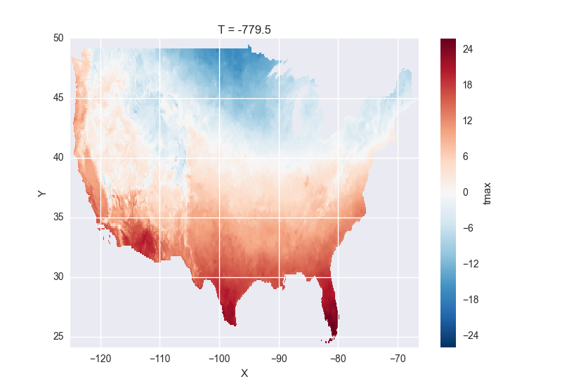
For example, we can open a connection to GBs of weather data produced by the PRISM project, and hosted by IRI at Columbia:

In [54]: remote_data = xr.open_dataset(
   ....:     "http://iridl.ldeo.columbia.edu/SOURCES/.OSU/.PRISM/.monthly/dods",
   ....:     decode_times=False,
   ....: )
   ....: 

In [55]: remote_data
Out[55]: 
<xarray.Dataset>
Dimensions:  (T: 1422, X: 1405, Y: 621)
Coordinates:
  * X        (X) float32 -125.0 -124.958 -124.917 -124.875 -124.833 -124.792 -124.75 ...
  * T        (T) float32 -779.5 -778.5 -777.5 -776.5 -775.5 -774.5 -773.5 -772.5 -771.5 ...
  * Y        (Y) float32 49.9167 49.875 49.8333 49.7917 49.75 49.7083 49.6667 49.625 ...
Data variables:
    ppt      (T, Y, X) float64 ...
    tdmean   (T, Y, X) float64 ...
    tmax     (T, Y, X) float64 ...
    tmin     (T, Y, X) float64 ...
Attributes:
    Conventions: IRIDL
    expires: 1375315200

Note

Like many real-world datasets, this dataset does not entirely follow CF conventions. Unexpected formats will usually cause xarray’s automatic decoding to fail. The way to work around this is to either set decode_cf=False in open_dataset to turn off all use of CF conventions, or by only disabling the troublesome parser. In this case, we set decode_times=False because the time axis here provides the calendar attribute in a format that xarray does not expect (the integer 360 instead of a string like '360_day').

We can select and slice this data any number of times, and nothing is loaded over the network until we look at particular values:

In [56]: tmax = remote_data["tmax"][:500, ::3, ::3]

In [57]: tmax
Out[57]: 
<xarray.DataArray 'tmax' (T: 500, Y: 207, X: 469)>
[48541500 values with dtype=float64]
Coordinates:
  * Y        (Y) float32 49.9167 49.7917 49.6667 49.5417 49.4167 49.2917 ...
  * X        (X) float32 -125.0 -124.875 -124.75 -124.625 -124.5 -124.375 ...
  * T        (T) float32 -779.5 -778.5 -777.5 -776.5 -775.5 -774.5 -773.5 ...
Attributes:
    pointwidth: 120
    standard_name: air_temperature
    units: Celsius_scale
    expires: 1443657600

# the data is downloaded automatically when we make the plot
In [58]: tmax[0].plot()

Some servers require authentication before we can access the data. For this purpose we can explicitly create a backends.PydapDataStore and pass in a Requests session object. For example for HTTP Basic authentication:

import xarray as xr
import requests

session = requests.Session()
session.auth = ('username', 'password')

store = xr.backends.PydapDataStore.open('http://example.com/data',
                                        session=session)
ds = xr.open_dataset(store)

Pydap’s cas module has functions that generate custom sessions for servers that use CAS single sign-on. For example, to connect to servers that require NASA’s URS authentication:

import xarray as xr
from pydata.cas.urs import setup_session

ds_url = 'https://gpm1.gesdisc.eosdis.nasa.gov/opendap/hyrax/example.nc'

session = setup_session('username', 'password', check_url=ds_url)
store = xr.backends.PydapDataStore.open(ds_url, session=session)

ds = xr.open_dataset(store)

Pickle

The simplest way to serialize an xarray object is to use Python’s built-in pickle module:

In [59]: import pickle

# use the highest protocol (-1) because it is way faster than the default
# text based pickle format
In [60]: pkl = pickle.dumps(ds, protocol=-1)

In [61]: pickle.loads(pkl)
Out[61]: 
<xarray.Dataset> Size: 62MB
Dimensions:  (time: 2920, lat: 25, lon: 53)
Coordinates:
  * time     (time) datetime64[ns] 23kB 2013-01-01 ... 2014-12-31T18:00:00
  * lat      (lat) float32 100B 75.0 72.5 70.0 67.5 65.0 ... 22.5 20.0 17.5 15.0
  * lon      (lon) float32 212B 200.0 202.5 205.0 207.5 ... 325.0 327.5 330.0
Data variables:
    dTdy     (time, lat, lon) float32 15MB dask.array<chunksize=(2920, 25, 53), meta=numpy.ma.MaskedArray>
    Tair     (time, lat, lon) float64 31MB dask.array<chunksize=(2920, 25, 53), meta=numpy.ma.MaskedArray>
    dTdx     (time, lat, lon) float32 15MB dask.array<chunksize=(2920, 25, 53), meta=numpy.ma.MaskedArray>
Attributes:
    description:  Data is from NMC initialized reanalysis\n(4x/day).  These a...
    platform:     Model
    references:   http://www.esrl.noaa.gov/psd/data/gridded/data.ncep.reanaly...
    title:        4x daily NMC reanalysis (1948)
    Conventions:  CF-1.7

Pickling is important because it doesn’t require any external libraries and lets you use xarray objects with Python modules like multiprocessing or Dask. However, pickling is not recommended for long-term storage.

Restoring a pickle requires that the internal structure of the types for the pickled data remain unchanged. Because the internal design of xarray is still being refined, we make no guarantees (at this point) that objects pickled with this version of xarray will work in future versions.

Note

When pickling an object opened from a NetCDF file, the pickle file will contain a reference to the file on disk. If you want to store the actual array values, load it into memory first with Dataset.load() or Dataset.compute().

Dictionary

We can convert a Dataset (or a DataArray) to a dict using Dataset.to_dict():

In [62]: ds = xr.Dataset({"foo": ("x", np.arange(30))})

In [63]: ds
Out[63]: 
<xarray.Dataset> Size: 240B
Dimensions:  (x: 30)
Dimensions without coordinates: x
Data variables:
    foo      (x) int64 240B 0 1 2 3 4 5 6 7 8 9 ... 21 22 23 24 25 26 27 28 29

In [64]: d = ds.to_dict()

In [65]: d
Out[65]: 
{'coords': {},
 'attrs': {},
 'dims': {'x': 30},
 'data_vars': {'foo': {'dims': ('x',),
   'attrs': {},
   'data': [0,
    1,
    2,
    3,
    4,
    5,
    6,
    7,
    8,
    9,
    10,
    11,
    12,
    13,
    14,
    15,
    16,
    17,
    18,
    19,
    20,
    21,
    22,
    23,
    24,
    25,
    26,
    27,
    28,
    29]}}}

We can create a new xarray object from a dict using Dataset.from_dict():

In [66]: ds_dict = xr.Dataset.from_dict(d)

In [67]: ds_dict
Out[67]: 
<xarray.Dataset> Size: 240B
Dimensions:  (x: 30)
Dimensions without coordinates: x
Data variables:
    foo      (x) int64 240B 0 1 2 3 4 5 6 7 8 9 ... 21 22 23 24 25 26 27 28 29

Dictionary support allows for flexible use of xarray objects. It doesn’t require external libraries and dicts can easily be pickled, or converted to json, or geojson. All the values are converted to lists, so dicts might be quite large.

To export just the dataset schema without the data itself, use the data=False option:

In [68]: ds.to_dict(data=False)
Out[68]: 
{'coords': {},
 'attrs': {},
 'dims': {'x': 30},
 'data_vars': {'foo': {'dims': ('x',),
   'attrs': {},
   'dtype': 'int64',
   'shape': (30,)}}}

This can be useful for generating indices of dataset contents to expose to search indices or other automated data discovery tools.

Rasterio

GDAL readable raster data using rasterio such as GeoTIFFs can be opened using the rioxarray extension. rioxarray can also handle geospatial related tasks such as re-projecting and clipping.

In [69]: import rioxarray

In [70]: rds = rioxarray.open_rasterio("RGB.byte.tif")

In [71]: rds
Out[71]: 
<xarray.DataArray (band: 3, y: 718, x: 791)>
[1703814 values with dtype=uint8]
Coordinates:
  * band         (band) int64 1 2 3
  * y            (y) float64 2.827e+06 2.826e+06 ... 2.612e+06 2.612e+06
  * x            (x) float64 1.021e+05 1.024e+05 ... 3.389e+05 3.392e+05
    spatial_ref  int64 0
Attributes:
    STATISTICS_MAXIMUM:  255
    STATISTICS_MEAN:     29.947726688477
    STATISTICS_MINIMUM:  0
    STATISTICS_STDDEV:   52.340921626611
    transform:           (300.0379266750948, 0.0, 101985.0, 0.0, -300.0417827...
    _FillValue:          0.0
    scale_factor:        1.0
    add_offset:          0.0
    grid_mapping:        spatial_ref

In [72]: rds.rio.crs
Out[72]: CRS.from_epsg(32618)

In [73]: rds4326 = rds.rio.reproject("epsg:4326")

In [74]: rds4326.rio.crs
Out[74]: CRS.from_epsg(4326)

In [75]: rds4326.rio.to_raster("RGB.byte.4326.tif")

GRIB format via cfgrib

Xarray supports reading GRIB files via ECMWF cfgrib python driver, if it is installed. To open a GRIB file supply engine='cfgrib' to open_dataset() after installing cfgrib:

In [76]: ds_grib = xr.open_dataset("example.grib", engine="cfgrib")

We recommend installing cfgrib via conda:

conda install -c conda-forge cfgrib

CSV and other formats supported by pandas

For more options (tabular formats and CSV files in particular), consider exporting your objects to pandas and using its broad range of IO tools. For CSV files, one might also consider xarray_extras.

Third party libraries

More formats are supported by extension libraries:

• xarray-mongodb: Store xarray objects on MongoDB