Working with Multidimensional Coordinates
Author: Ryan Abernathey
Many datasets have physical coordinates which differ from their logical coordinates. Xarray provides several ways to plot and analyze such datasets.
In [1]: import numpy as np

In [2]: import pandas as pd

In [3]: import xarray as xr

In [4]: import netCDF4

In [5]: import cartopy.crs as ccrs

In [6]: import matplotlib.pyplot as plt
As an example, consider this dataset from the xarray-data repository.
In [7]: ds = xr.tutorial.open_dataset('rasm').load()

In [8]: ds
Out[8]:
<xarray.Dataset>
Dimensions:  (time: 36, x: 275, y: 205)
Coordinates:
  * time     (time) object 1980-09-16 12:00:00 ... 1983-08-17 00:00:00
    xc       (y, x) float64 189.2 189.4 189.6 189.7 ... 17.65 17.4 17.15 16.91
    yc       (y, x) float64 16.53 16.78 17.02 17.27 ... 28.26 28.01 27.76 27.51
Dimensions without coordinates: x, y
Data variables:
    Tair     (time, y, x) float64 nan nan nan nan nan ... 29.8 28.66 28.19 28.21
Attributes:
    title:                     /workspace/jhamman/processed/R1002RBRxaaa01a/l...
    institution:               U.W.
    source:                    RACM R1002RBRxaaa01a
    output_frequency:          daily
    output_mode:               averaged
    convention:                CF-1.4
    references:                Based on the initial model of Liang et al., 19...
    comment:                   Output from the Variable Infiltration Capacity...
    nco_openmp_thread_number:  1
    NCO:                       "4.6.0"
    history:                   Tue Dec 27 14:15:22 2016: ncatted -a dimension...
In this example, the logical coordinates are x and y, while
the physical coordinates are xc and yc, which represent the
latitudes and longitude of the data.
In [9]: ds.xc.attrs
Out[9]:
{'long_name': 'longitude of grid cell center',
 'units': 'degrees_east',
 'bounds': 'xv'}

In [10]: ds.yc.attrs
Out[10]:
{'long_name': 'latitude of grid cell center',
 'units': 'degrees_north',
 'bounds': 'yv'}
Plotting
Let’s examine these coordinate variables by plotting them.
In [11]: fig, (ax1, ax2) = plt.subplots(ncols=2, figsize=(9,3))

In [12]: ds.xc.plot(ax=ax1);

In [13]: ds.yc.plot(ax=ax2);
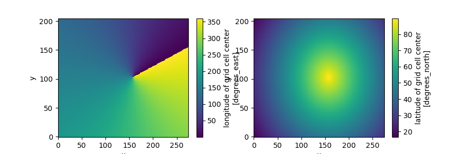
Note that the variables xc (longitude) and yc (latitude) are
two-dimensional scalar fields.
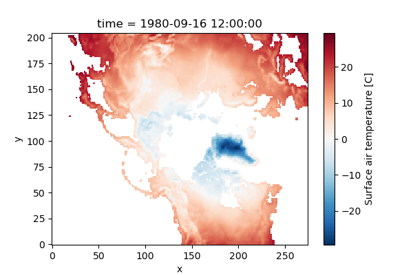
If we try to plot the data variable Tair, by default we get the
logical coordinates.
In [14]: ds.Tair[0].plot();
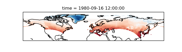
In order to visualize the data on a conventional latitude-longitude grid, we can take advantage of xarray’s ability to apply cartopy map projections.
In [15]: plt.figure(figsize=(7,2));

In [16]: ax = plt.axes(projection=ccrs.PlateCarree());

In [17]: ds.Tair[0].plot.pcolormesh(ax=ax, transform=ccrs.PlateCarree(),
   ....:                            x='xc', y='yc', add_colorbar=False);
   ....:

In [18]: ax.coastlines();
Multidimensional Groupby
The above example allowed us to visualize the data on a regular
latitude-longitude grid. But what if we want to do a calculation that
involves grouping over one of these physical coordinates (rather than
the logical coordinates), for example, calculating the mean temperature
at each latitude. This can be achieved using xarray’s groupby
function, which accepts multidimensional variables. By default,
groupby will use every unique value in the variable, which is
probably not what we want. Instead, we can use the groupby_bins
function to specify the output coordinates of the group.
# define two-degree wide latitude bins
In [19]: lat_bins = np.arange(0, 91, 2)

# define a label for each bin corresponding to the central latitude
In [20]: lat_center = np.arange(1, 90, 2)

# group according to those bins and take the mean
In [21]: Tair_lat_mean = (ds.Tair.groupby_bins('xc', lat_bins, labels=lat_center)
   ....:                  .mean(xr.ALL_DIMS))
   ....:

# plot the result
In [22]: Tair_lat_mean.plot();
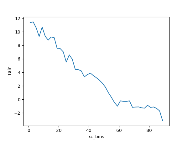
Note that the resulting coordinate for the groupby_bins operation
got the _bins suffix appended: xc_bins. This help us distinguish
it from the original multidimensional variable xc.