Out of core computation with dask
xray v0.5 includes experimental integration with dask to support streaming computation on datasets that don’t fit into memory.
Currently, dask is an entirely optional feature for xray. However, the benefits of using dask are sufficiently strong that we expect that dask may become a requirement for a future version of xray.
What is a dask array?
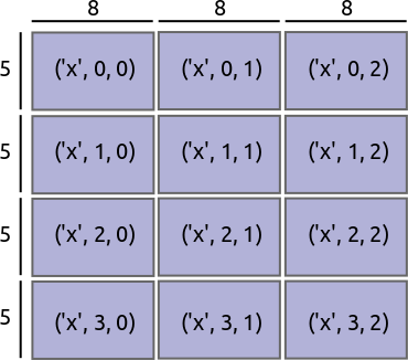
Dask divides arrays into many small pieces, called chunks, each of which is presumed to be small enough to fit into memory.
Unlike NumPy, which has eager evaluation, operations on dask arrays are lazy. Operations queue up a series of taks mapped over blocks, and no computation is performed until you actually ask values to be computed (e.g., to print results to your screen or write to disk). At that point, data is loaded into memory and computation proceeds in a streaming fashion, block-by-block.
The actual computation is controlled by a multi-processing or thread pool, which allows dask to take full advantage of multiple processers available on most modern computers.
For more details on dask, read its documentation.
Reading and writing data
The usual way to create a dataset filled with dask arrays is to load the data from a netCDF file or files. You can by supplying a chunks argument to open_dataset() or using the open_mfdataset() function.
In [1]: ds = xray.open_dataset('example-data.nc', chunks={'time': 10})

In [2]: ds
Out[2]:
<xray.Dataset>
Dimensions:      (latitude: 180, longitude: 360, time: 365)
Coordinates:
  * latitude     (latitude) >f4 89.5 88.5 87.5 86.5 85.5 84.5 83.5 82.5 81.5 ...
  * time         (time) datetime64[ns] 2015-01-01 2015-01-02 2015-01-03 ...
  * longitude    (longitude) int64 0 1 2 3 4 5 6 7 8 9 10 11 12 13 14 15 16 ...
Data variables:
    temperature  (time, latitude, longitude) >f4 0.469112 -0.282863 -1.50906 ...
If you don’t supply a dimension in chunks, only one chunk will be used along that dimension for all dask arrays in the dataset. It is also entirely equivalent to open a dataset using open_dataset and then chunk the data use the chunk method, e.g., xray.open_dataset('example-data.nc').chunk({'time': 10}).
To open multiple files simultaneously, use open_mfdataset():
xray.open_mfdataset('my/files/*.nc')
This function will automatically concatenate and merge dataset into one in the simple cases that it understands (see auto_combine() for the full disclaimer). By default, open_mfdataset will chunk each netCDF file into a single dask array; again, supply the chunks argument to control the size of the resulting dask arrays. In more complex cases, you can open each file individually using open_dataset and merge the result, as described in Combining data.
You’ll notice that printing a dataset still shows a preview of array values, even if they are actually dask arrays. We can do this quickly with dask because we only need to the compute the first few values (typically from the first block). To reveal the true nature of an array, print a DataArray:
In [3]: ds.temperature
Out[3]:
<xray.DataArray 'temperature' (time: 365, latitude: 180, longitude: 360)>
dask.array<xray_temperature_1, shape=(365, 180, 360), chunks=((10, 10, 10, ..., 10, 5), (180,), (360,)), dtype=>f4>
Coordinates:
  * latitude   (latitude) >f4 89.5 88.5 87.5 86.5 85.5 84.5 83.5 82.5 81.5 ...
  * longitude  (longitude) int64 0 1 2 3 4 5 6 7 8 9 10 11 12 13 14 15 16 17 ...
  * time       (time) datetime64[ns] 2015-01-01 2015-01-02 2015-01-03 ...
Once you’ve manipulated a dask array, you can still write a dataset too big to fit into memory back to disk by using to_netcdf() in the usual way.
Using dask with xray
Nearly all existing xray methods (including those for indexing, computation, concatenating and grouped operations) have been extended to work automatically with dask arrays. When you load data as a dask array in an xray data structure, almost all xray operations will keep it as a dask array; when this is not possible, they will raise an exception rather than unexpectedly loading data into memory. Converting a dask array into memory generally requires an explicit conversion step. One noteable exception is indexing operations: to enable label based indexing, xray will automatically load coordinate labels into memory.
The easiest way to convert an xray data structure from lazy dask arrays into eager, in-memory numpy arrays is to use the load() method:
In [4]: ds.load()
Out[4]:
<xray.Dataset>
Dimensions:      (latitude: 180, longitude: 360, time: 365)
Coordinates:
  * latitude     (latitude) >f4 89.5 88.5 87.5 86.5 85.5 84.5 83.5 82.5 81.5 ...
  * time         (time) datetime64[ns] 2015-01-01 2015-01-02 2015-01-03 ...
  * longitude    (longitude) int64 0 1 2 3 4 5 6 7 8 9 10 11 12 13 14 15 16 ...
Data variables:
    temperature  (time, latitude, longitude) float32 0.469112 -0.282863 ...
You can also access values, which will always be a numpy array:
In [5]: ds.temperature.values
Out[5]:
array([[[  4.691e-01,  -2.829e-01, ...,  -5.577e-01,   3.814e-01],
        [  1.337e+00,  -1.531e+00, ...,   8.726e-01,  -1.538e+00],
        ...
# truncated for brevity
Explicit conversion by wrapping a DataArray with np.asarray also works:
In [6]: np.asarray(ds.temperature)
Out[6]:
array([[[  4.691e-01,  -2.829e-01, ...,  -5.577e-01,   3.814e-01],
        [  1.337e+00,  -1.531e+00, ...,   8.726e-01,  -1.538e+00],
        ...
With the current versions of xray and dask, there is no automatic conversion of eager numpy arrays to dask arrays, nor automatic alignment of chunks when performing operations between dask arrays with different chunk sizes. You will need to explicitly chunk each array to ensure compatibility. With xray, both converting data to a dask arrays and converting the chunk sizes of dask arrays is done with the chunk() method:
In [7]: rechunked = ds.chunk({'latitude': 100, 'longitude': 100})
You can view the size of existing chunks on an array by viewing the chunks attribute:
In [8]: rechunked.chunks
Out[8]: Frozen(SortedKeysDict({'latitude': (100, 80), 'longitude': (100, 100, 100, 60), 'time': (10, 10, 10, 10, 10, 10, 10, 10, 10, 10, 10, 10, 10, 10, 10, 10, 10, 10, 10, 10, 10, 10, 10, 10, 10, 10, 10, 10, 10, 10, 10, 10, 10, 10, 10, 10, 5)}))
If there are not consistent chunksizes between all the ararys in a dataset along a particular dimension, an exception is raised when you try to access .chunks.
Note
In the future, we would like to enable automatic alignment of dask chunksizes and automatic conversion of numpy arrays to dask (but not the other way around). We might also require that all arrays in a dataset share the same chunking alignment. None of these are currently done.
NumPy ufuncs like np.sin currently only work on eagerly evaluated arrays (this will change with the next major NumPy release). We have provided replacements that also work on all xray objects, including those that store lazy dask arrays, in the xray.ufuncs module:
In [9]: import xray.ufuncs as xu

In [10]: xu.sin(rechunked)
Out[10]:
<xray.Dataset>
Dimensions:      (latitude: 180, longitude: 360, time: 365)
Coordinates:
  * latitude     (latitude) >f4 89.5 88.5 87.5 86.5 85.5 84.5 83.5 82.5 81.5 ...
  * longitude    (longitude) int64 0 1 2 3 4 5 6 7 8 9 10 11 12 13 14 15 16 ...
  * time         (time) datetime64[ns] 2015-01-01 2015-01-02 2015-01-03 ...
Data variables:
    temperature  (time, latitude, longitude) float32 0.452095 -0.279106 ...
To access dask arrays directly, use the new DataArray.data attribute. This attribute exposes array data either as a dask array or as a numpy array, depending on whether it has been loaded into dask or not:
In [11]: ds.temperature.data
Out[11]: dask.array<xray_temperature_5, shape=(365, 180, 360), chunks=((10, 10, 10, ..., 10, 5), (180,), (360,)), dtype=float32>
Note
In the future, we may extend .data to support other “computable” array backends beyond dask and numpy (e.g., to support sparse arrays).
Chunking and performance
The chunks parameter has critical performance implications when using dask arrays. If your chunks are too small, queueing up operations will be extremely slow, because dask will translates each operation into a huge number of operations mapped across chunks. Computation on dask arrays with small chunks can also be slow, because each operation on a chunk has some fixed overhead from the Python interpreter and the dask task executor.
Conversely, if your chunks are too big, some of your computation may be wasted, because dask only computes results one chunk at a time.
A good rule of thumb to create arrays with a minimum chunksize of at least one million elements (e.g., a 1000x1000 matrix). With large arrays (10+ GB), the cost of queueing up dask operations can be noticeable, and you may need even larger chunksizes.