You can run this notebook in a live session on Github .
ROMS Ocean Model Example
The Regional Ocean Modeling System (ROMS ) is an open source hydrodynamic model that is used for simulating currents and water properties in coastal and estuarine regions. ROMS is one of a few standard ocean models, and it has an active user community.
ROMS uses a regular C-Grid in the horizontal, similar to other structured grid ocean and atmospheric models, and a stretched vertical coordinate (see the ROMS documentation for more details). Both of these require special treatment when using xarray xgcm
Load a sample ROMS file. This is a subset of a full model available at
The subsetting was done using the following command on one of the output files:
So, the ROMS_example.nc
Load in ROMS dataset as an xarray object
<xarray.Dataset> Size: 19MB
Dimensions:     (ocean_time: 2, s_rho: 30, eta_rho: 191, xi_rho: 371)
Coordinates:
  * ocean_time  (ocean_time) datetime64[ns] 16B 2001-08-01 2001-08-08
  * s_rho       (s_rho) float64 240B -0.9833 -0.95 -0.9167 ... -0.05 -0.01667
    Cs_r        (s_rho) float64 240B dask.array<chunksize=(30,), meta=np.ndarray>
    lon_rho     (eta_rho, xi_rho) float64 567kB dask.array<chunksize=(191, 371), meta=np.ndarray>
    h           (eta_rho, xi_rho) float64 567kB dask.array<chunksize=(191, 371), meta=np.ndarray>
    lat_rho     (eta_rho, xi_rho) float64 567kB dask.array<chunksize=(191, 371), meta=np.ndarray>
    hc          float64 8B ...
    Vtransform  int32 4B ...
Dimensions without coordinates: eta_rho, xi_rho
Data variables:
    salt        (ocean_time, s_rho, eta_rho, xi_rho) float32 17MB dask.array<chunksize=(1, 15, 96, 186), meta=np.ndarray>
    zeta        (ocean_time, eta_rho, xi_rho) float32 567kB dask.array<chunksize=(1, 191, 371), meta=np.ndarray>
Attributes: (12/34)
    file:              ../output_20yr_obc/2001/ocean_his_0015.nc
    format:            netCDF-4/HDF5 file
    Conventions:       CF-1.4
    type:              ROMS/TOMS history file
    title:             TXLA ROMS hindcast run with dyes and oxygen
    rst_file:          ../output_20yr_obc/2001/ocean_rst.nc
    ...                ...
    compiler_flags:    -heap-arrays -fp-model fast -mt_mpi -ip -O3 -msse2 -free
    tiling:            010x012
    history:           Tue Jul 24 11:04:43 2018: /opt/nco/ncks -D 4 -t 8 /cop...
    ana_file:          /home/d.kobashi/TXLA_ROMS_reana/Functionals/ana_btflux...
    CPP_options:       TXLA2, ANA_BPFLUX, ANA_BSFLUX, ANA_BTFLUX, ANA_NUDGCOE...
NCO: netCDF Operators version 4.7.6-alpha04 (Homepage = htt... Dimensions: ocean_time : 2s_rho : 30eta_rho : 191xi_rho : 371Coordinates: (8)
ocean_time
(ocean_time)
datetime64[ns]
2001-08-01 2001-08-08
long_name : time since initialization field : time, scalar, series array(['2001-08-01T00:00:00.000000000', '2001-08-08T00:00:00.000000000'],
dtype='datetime64[ns]') s_rho
(s_rho)
float64
-0.9833 -0.95 ... -0.05 -0.01667
long_name : S-coordinate at RHO-points valid_min : -1.0 valid_max : 0.0 positive : up standard_name : ocean_s_coordinate_g2 formula_terms : s: s_rho C: Cs_r eta: zeta depth: h depth_c: hc field : s_rho, scalar array([-0.983333, -0.95 , -0.916667, -0.883333, -0.85 , -0.816667,
-0.783333, -0.75 , -0.716667, -0.683333, -0.65 , -0.616667,
-0.583333, -0.55 , -0.516667, -0.483333, -0.45 , -0.416667,
-0.383333, -0.35 , -0.316667, -0.283333, -0.25 , -0.216667,
-0.183333, -0.15 , -0.116667, -0.083333, -0.05 , -0.016667]) Cs_r
(s_rho)
float64
dask.array<chunksize=(30,), meta=np.ndarray>
long_name : S-coordinate stretching curves at RHO-points valid_min : -1.0 valid_max : 0.0 field : Cs_r, scalar
Array
Chunk
Bytes
240 B
240 B
Shape
(30,)
(30,)
Dask graph
1 chunks in 2 graph layers
Data type
float64 numpy.ndarray
30
1
lon_rho
(eta_rho, xi_rho)
float64
dask.array<chunksize=(191, 371), meta=np.ndarray>
long_name : longitude of RHO-points units : degree_east standard_name : longitude field : lon_rho, scalar
Array
Chunk
Bytes
553.60 kiB
553.60 kiB
Shape
(191, 371)
(191, 371)
Dask graph
1 chunks in 2 graph layers
Data type
float64 numpy.ndarray
371
191
h
(eta_rho, xi_rho)
float64
dask.array<chunksize=(191, 371), meta=np.ndarray>
long_name : bathymetry at RHO-points units : meter field : bath, scalar
Array
Chunk
Bytes
553.60 kiB
553.60 kiB
Shape
(191, 371)
(191, 371)
Dask graph
1 chunks in 2 graph layers
Data type
float64 numpy.ndarray
371
191
lat_rho
(eta_rho, xi_rho)
float64
dask.array<chunksize=(191, 371), meta=np.ndarray>
long_name : latitude of RHO-points units : degree_north standard_name : latitude field : lat_rho, scalar
Array
Chunk
Bytes
553.60 kiB
553.60 kiB
Shape
(191, 371)
(191, 371)
Dask graph
1 chunks in 2 graph layers
Data type
float64 numpy.ndarray
371
191
hc
()
float64
...
long_name : S-coordinate parameter, critical depth units : meter [1 values with dtype=float64] Vtransform
()
int32
...
long_name : vertical terrain-following transformation equation [1 values with dtype=int32] Data variables: (2)
salt
(ocean_time, s_rho, eta_rho, xi_rho)
float32
dask.array<chunksize=(1, 15, 96, 186), meta=np.ndarray>
long_name : salinity time : ocean_time field : salinity, scalar, series
Array
Chunk
Bytes
16.22 MiB
1.02 MiB
Shape
(2, 30, 191, 371)
(1, 15, 96, 186)
Dask graph
16 chunks in 2 graph layers
Data type
float32 numpy.ndarray
2
1
371
191
30
zeta
(ocean_time, eta_rho, xi_rho)
float32
dask.array<chunksize=(1, 191, 371), meta=np.ndarray>
long_name : free-surface units : meter time : ocean_time field : free-surface, scalar, series
Array
Chunk
Bytes
553.60 kiB
276.80 kiB
Shape
(2, 191, 371)
(1, 191, 371)
Dask graph
2 chunks in 2 graph layers
Data type
float32 numpy.ndarray
371
191
2
Attributes: (34)
file : ../output_20yr_obc/2001/ocean_his_0015.nc format : netCDF-4/HDF5 file Conventions : CF-1.4 type : ROMS/TOMS history file title : TXLA ROMS hindcast run with dyes and oxygen rst_file : ../output_20yr_obc/2001/ocean_rst.nc his_base : ../output_20yr_obc/2001/ocean_his avg_base : ../output_20yr_obc/2001/ocean_avg dia_base : ../output_20yr_obc/2001/ocean_dia sta_file : ocean_sta.nc grd_file : ../inputs/grd/txla2_grd_v4_test_lcut_hglo_wtype.nc ini_file : ../output_20yr_obc/2000/ocean_rst.nc frc_file_01 : ../inputs/2001/txla_bulk_ERAI_2001.nc frc_file_02 : ../inputs/2001/txla_flx_ICOADS_AVHRR_SST_2001.nc, ../inputs/2002/txla_flx_ICOADS_AVHRR_SST_2002.nc bry_file_01 : ../inputs/2001/txla2_bry_2001_glo_ReAna_v4_o2woa.nc, ../inputs/2002/txla2_bry_2002_glo_ReAna_v4_o2woa.nc clm_file_01 : ../inputs/2001/txla2_clm_2001_01_glo_ReAna_v4_o2woa.nc, ../inputs/2001/txla2_clm_2001_02_glo_ReAna_v4_o2woa.nc, ../inputs/2001/txla2_clm_2001_03_glo_ReAna_v4_o2woa.nc, ../inputs/2001/txla2_clm_2001_04_glo_ReAna_v4_o2woa.nc, ../inputs/2001/txla2_clm_2001_05_glo_ReAna_v4_o2woa.nc, ../inputs/2001/txla2_clm_2001_06_glo_ReAna_v4_o2woa.nc, ../inputs/2001/txla2_clm_2001_07_glo_ReAna_v4_o2woa.nc, ../inputs/2001/txla2_clm_2001_08_glo_ReAna_v4_o2woa.nc, ../inputs/2001/txla2_clm_2001_09_glo_ReAna_v4_o2woa.nc, ../inputs/2001/txla2_clm_2001_10_glo_ReAna_v4_o2woa.nc, ../inputs/2001/txla2_clm_2001_11_glo_ReAna_v4_o2woa.nc, ../inputs/2001/txla2_clm_2001_12_glo_ReAna_v4_o2woa.nc, ../inputs/2002/txla2_clm_2002_01_glo_ReAna_v4_o2woa.nc script_file : spos_file : /scratch/user/d.kobashi/inputs/stations.in NLM_LBC :
EDGE: WEST SOUTH EAST NORTH
zeta: Che Che Che Clo
ubar: Shc Shc Shc Clo
vbar: Shc Shc Shc Clo
u: Rad Rad Rad Clo
v: Rad Rad Rad Clo
temp: Rad Rad Rad Clo
salt: Rad Rad Rad Clo
dye_01: Gra Gra Gra Clo
dye_02: Rad Rad Rad Clo
dye_03: Rad Rad Rad Clo
dye_04: Rad Rad Rad Clo
tke: Gra Gra Gra Clo svn_url : https:://myroms.org/svn/src svn_rev : code_dir : /scratch/user/d.kobashi/source_code/COAWST/COAWST.r960-dev header_dir : /home/d.kobashi/TXLA_ROMS_reana/work_20yr_obc header_file : txla2.h os : Linux cpu : x86_64 compiler_system : ifort compiler_command : /software/easybuild/software/impi/5.0.1.035-iccifort-2015.0.090/bin64/mpiifort compiler_flags : -heap-arrays -fp-model fast -mt_mpi -ip -O3 -msse2 -free tiling : 010x012 history : Tue Jul 24 11:04:43 2018: /opt/nco/ncks -D 4 -t 8 /copano/d1/shared/TXLA_ROMS/output_20yr_obc/2001/ocean_his_0015.nc --cnk_dmn ocean_time,4 --cnk_dmn eta_rho,8 --cnk_dmn eta_u,8 --cnk_dmn eta_v,8 --cnk_dmn eta_psi,8 --cnk_dmn xi_rho,16 --cnk_dmn xi_u,16 --cnk_dmn xi_v,16 --cnk_dmn xi_psi,16 --cnk_dmn s_rho,2 --cnk_dmn s_w,2 --output /copano/d2/shared/TXLA_ROMS/output_20yr_obc/2001/ocean_his_0015.nc
ROMS/TOMS, Version 3.7, Monday - July 18, 2016 - 10:38:26 PM ana_file : /home/d.kobashi/TXLA_ROMS_reana/Functionals/ana_btflux.h, /home/d.kobashi/TXLA_ROMS_reana/Functionals/ana_sponge.h, /home/d.kobashi/TXLA_ROMS_reana/Functionals/ana_nudgcoef.h, /home/d.kobashi/TXLA_ROMS_reana/Functionals/ana_stflux.h CPP_options : TXLA2, ANA_BPFLUX, ANA_BSFLUX, ANA_BTFLUX, ANA_NUDGCOEF, ANA_SPFLUX, ANA_SPONGE, ASSUMED_SHAPE, AVERAGES, BULK_FLUXES, CURVGRID, DEFLATE, DIAGNOSTICS_TS, DIAGNOSTICS_UV, DIFF_GRID, DJ_GRADPS, DOUBLE_PRECISION, EMINUSP, GLS_MIXING, HDF5, KANTHA_CLAYSON, LONGWAVE, MASKING, MIX_GEO_TS, MIX_S_UV, MPI, NONLINEAR, NONLIN_EOS, N2S2_HORAVG, POWER_LAW, PROFILE, QCORRECTION, K_GSCHEME, RADIATION_2D, !RST_SINGLE, SALINITY, SOLAR_SOURCE, SOLVE3D, SPLINES, SPHERICAL, STATIONS, T_PASSIVE, TS_MPDATA, TS_DIF2, UV_ADV, UV_COR, UV_U3HADVECTION, UV_C4VADVECTION, UV_LOGDRAG, UV_VIS2, VAR_RHO_2D, VISC_GRID, WTYPE_GRID NCO : netCDF Operators version 4.7.6-alpha04 (Homepage = http://nco.sf.net, Code = http://github.com/nco/nco)
Add a lazilly calculated vertical coordinates
Write equations to calculate the vertical coordinate. These will be only evaluated when data is requested. Information about the ROMS vertical coordinate can be found here .
In short, for Vtransform==2
\(Z_0 = (h_c \, S + h \,C) / (h_c + h)\)
\(z = Z_0 (\zeta + h) + \zeta\)
where the variables are defined as in the link above.
<xarray.DataArray 'salt' (ocean_time: 2, s_rho: 30, eta_rho: 191, xi_rho: 371)> Size: 17MB
dask.array<open_dataset-salt, shape=(2, 30, 191, 371), dtype=float32, chunksize=(1, 15, 96, 186), chunktype=numpy.ndarray>
Coordinates:
  * ocean_time  (ocean_time) datetime64[ns] 16B 2001-08-01 2001-08-08
    z_rho       (s_rho, xi_rho, eta_rho, ocean_time) float64 34MB dask.array<chunksize=(30, 371, 191, 1), meta=np.ndarray>
  * s_rho       (s_rho) float64 240B -0.9833 -0.95 -0.9167 ... -0.05 -0.01667
    Cs_r        (s_rho) float64 240B dask.array<chunksize=(30,), meta=np.ndarray>
    lon_rho     (xi_rho, eta_rho) float64 567kB dask.array<chunksize=(371, 191), meta=np.ndarray>
    h           (xi_rho, eta_rho) float64 567kB dask.array<chunksize=(371, 191), meta=np.ndarray>
    lat_rho     (xi_rho, eta_rho) float64 567kB dask.array<chunksize=(371, 191), meta=np.ndarray>
    hc          float64 8B ...
    Vtransform  int32 4B ...
Dimensions without coordinates: eta_rho, xi_rho
Attributes:
    long_name:  salinity
    time:       ocean_time
field: salinity, scalar, series dask.array<chunksize=(1, 15, 96, 186), meta=np.ndarray>
Array
Chunk
Bytes
16.22 MiB
1.02 MiB
Shape
(2, 30, 191, 371)
(1, 15, 96, 186)
Dask graph
16 chunks in 2 graph layers
Data type
float32 numpy.ndarray
2
1
371
191
30
Coordinates: (9)
ocean_time
(ocean_time)
datetime64[ns]
2001-08-01 2001-08-08
long_name : time since initialization field : time, scalar, series array(['2001-08-01T00:00:00.000000000', '2001-08-08T00:00:00.000000000'],
dtype='datetime64[ns]') z_rho
(s_rho, xi_rho, eta_rho, ocean_time)
float64
dask.array<chunksize=(30, 371, 191, 1), meta=np.ndarray>
long_name : free-surface units : meter time : ocean_time field : free-surface, scalar, series valid_min : -1.0 valid_max : 0.0 positive : up standard_name : ocean_s_coordinate_g2 formula_terms : s: s_rho C: Cs_r eta: zeta depth: h depth_c: hc
Array
Chunk
Bytes
32.44 MiB
16.22 MiB
Shape
(30, 371, 191, 2)
(30, 371, 191, 1)
Dask graph
2 chunks in 26 graph layers
Data type
float64 numpy.ndarray
30
1
2
191
371
s_rho
(s_rho)
float64
-0.9833 -0.95 ... -0.05 -0.01667
long_name : S-coordinate at RHO-points valid_min : -1.0 valid_max : 0.0 positive : up standard_name : ocean_s_coordinate_g2 formula_terms : s: s_rho C: Cs_r eta: zeta depth: h depth_c: hc field : s_rho, scalar array([-0.983333, -0.95 , -0.916667, -0.883333, -0.85 , -0.816667,
-0.783333, -0.75 , -0.716667, -0.683333, -0.65 , -0.616667,
-0.583333, -0.55 , -0.516667, -0.483333, -0.45 , -0.416667,
-0.383333, -0.35 , -0.316667, -0.283333, -0.25 , -0.216667,
-0.183333, -0.15 , -0.116667, -0.083333, -0.05 , -0.016667]) Cs_r
(s_rho)
float64
dask.array<chunksize=(30,), meta=np.ndarray>
long_name : S-coordinate stretching curves at RHO-points valid_min : -1.0 valid_max : 0.0 field : Cs_r, scalar
Array
Chunk
Bytes
240 B
240 B
Shape
(30,)
(30,)
Dask graph
1 chunks in 2 graph layers
Data type
float64 numpy.ndarray
30
1
lon_rho
(xi_rho, eta_rho)
float64
dask.array<chunksize=(371, 191), meta=np.ndarray>
long_name : longitude of RHO-points units : degree_east standard_name : longitude field : lon_rho, scalar
Array
Chunk
Bytes
553.60 kiB
553.60 kiB
Shape
(371, 191)
(371, 191)
Dask graph
1 chunks in 3 graph layers
Data type
float64 numpy.ndarray
191
371
h
(xi_rho, eta_rho)
float64
dask.array<chunksize=(371, 191), meta=np.ndarray>
long_name : bathymetry at RHO-points units : meter field : bath, scalar
Array
Chunk
Bytes
553.60 kiB
553.60 kiB
Shape
(371, 191)
(371, 191)
Dask graph
1 chunks in 3 graph layers
Data type
float64 numpy.ndarray
191
371
lat_rho
(xi_rho, eta_rho)
float64
dask.array<chunksize=(371, 191), meta=np.ndarray>
long_name : latitude of RHO-points units : degree_north standard_name : latitude field : lat_rho, scalar
Array
Chunk
Bytes
553.60 kiB
553.60 kiB
Shape
(371, 191)
(371, 191)
Dask graph
1 chunks in 3 graph layers
Data type
float64 numpy.ndarray
191
371
hc
()
float64
...
long_name : S-coordinate parameter, critical depth units : meter [1 values with dtype=float64] Vtransform
()
int32
...
long_name : vertical terrain-following transformation equation [1 values with dtype=int32] Attributes: (3)
long_name : salinity time : ocean_time field : salinity, scalar, series
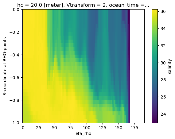
A naive vertical slice
Creating a slice using the s-coordinate as the vertical dimension is typically not very informative.
<matplotlib.collections.QuadMesh at 0x78b3ddb4c440>
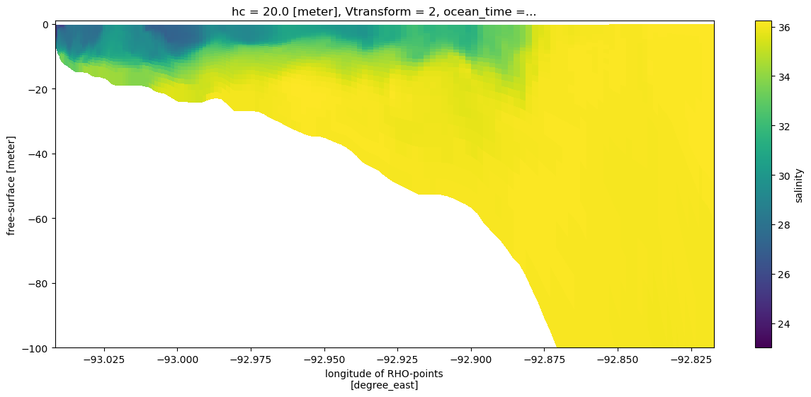
We can feed coordinate information to the plot method to give a more informative cross-section that uses the depths. Note that we did not need to slice the depth or longitude information separately, this was done automatically as the variable was sliced.
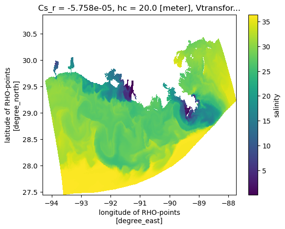
A plan view
Now make a naive plan view, without any projection information, just using lon/lat as x/y. This looks OK, but will appear compressed because lon and lat do not have an aspect constrained by the projection.
<matplotlib.collections.QuadMesh at 0x78b3dcab2990>
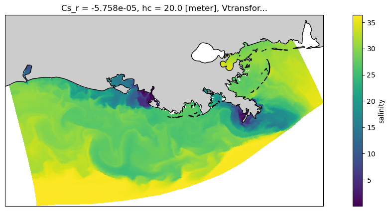
And let’s use a projection to make it nicer, and add a coast.
<cartopy.mpl.feature_artist.FeatureArtist at 0x78b3dca56e40>
/home/docs/checkouts/readthedocs.org/user_builds/xray/checkouts/stable/.pixi/envs/doc/lib/python3.14/site-packages/cartopy/io/__init__.py:242: DownloadWarning: Downloading: https://naturalearth.s3.amazonaws.com/10m_physical/ne_10m_land.zip
  warnings.warn(f'Downloading: {url}', DownloadWarning)