Toy weather data
Contents
You can run this notebook in a live session ![]() or view it on Github.
or view it on Github.
Toy weather data#
Here is an example of how to easily manipulate a toy weather dataset using xarray and other recommended Python libraries:
[1]:
import numpy as np
import pandas as pd
import seaborn as sns

import xarray as xr

np.random.seed(123)

xr.set_options(display_style="html")

times = pd.date_range("2000-01-01", "2001-12-31", name="time")
annual_cycle = np.sin(2 * np.pi * (times.dayofyear.values / 365.25 - 0.28))

base = 10 + 15 * annual_cycle.reshape(-1, 1)
tmin_values = base + 3 * np.random.randn(annual_cycle.size, 3)
tmax_values = base + 10 + 3 * np.random.randn(annual_cycle.size, 3)

ds = xr.Dataset(
    {
        "tmin": (("time", "location"), tmin_values),
        "tmax": (("time", "location"), tmax_values),
    },
    {"time": times, "location": ["IA", "IN", "IL"]},
)

ds
[1]:
<xarray.Dataset>
Dimensions:   (time: 731, location: 3)
Coordinates:
  * time      (time) datetime64[ns] 2000-01-01 2000-01-02 ... 2001-12-31
  * location  (location) <U2 'IA' 'IN' 'IL'
Data variables:
    tmin      (time, location) float64 -8.037 -1.788 -3.932 ... -1.346 -4.544
tmax (time, location) float64 12.98 3.31 6.779 ... 6.636 3.343 3.805Examine a dataset with pandas and seaborn#
Convert to a pandas DataFrame#
[2]:
df = ds.to_dataframe()
df.head()
[2]:
| tmin | tmax | ||
|---|---|---|---|
| time | location | ||
| 2000-01-01 | IA | -8.037369 | 12.980549 |
| IN | -1.788441 | 3.310409 | |
| IL | -3.931542 | 6.778554 | |
| 2000-01-02 | IA | -9.341157 | 0.447856 |
| IN | -6.558073 | 6.372712 |
[3]:
df.describe()
[3]:
| tmin | tmax | |
|---|---|---|
| count | 2193.000000 | 2193.000000 |
| mean | 9.975426 | 20.108232 |
| std | 10.963228 | 11.010569 |
| min | -13.395763 | -3.506234 |
| 25% | -0.040347 | 9.853905 |
| 50% | 10.060403 | 19.967409 |
| 75% | 20.083590 | 30.045588 |
| max | 33.456060 | 43.271148 |
Visualize using pandas#
[4]:
ds.mean(dim="location").to_dataframe().plot()
[4]:
<AxesSubplot: xlabel='time'>
Visualize using seaborn#
[5]:
sns.pairplot(df.reset_index(), vars=ds.data_vars)
---------------------------------------------------------------------------
StopIteration                             Traceback (most recent call last)
Cell In [5], line 1
----> 1 sns.pairplot(df.reset_index(), vars=ds.data_vars)

File ~/checkouts/readthedocs.org/user_builds/xray/conda/v2022.10.0/lib/python3.9/site-packages/seaborn/axisgrid.py:2144, in pairplot(data, hue, hue_order, palette, vars, x_vars, y_vars, kind, diag_kind, markers, height, aspect, corner, dropna, plot_kws, diag_kws, grid_kws, size)
   2142 diag_kws.setdefault("legend", False)
   2143 if diag_kind == "hist":
-> 2144     grid.map_diag(histplot, **diag_kws)
   2145 elif diag_kind == "kde":
   2146     diag_kws.setdefault("fill", True)

File ~/checkouts/readthedocs.org/user_builds/xray/conda/v2022.10.0/lib/python3.9/site-packages/seaborn/axisgrid.py:1507, in PairGrid.map_diag(self, func, **kwargs)
   1505     plot_kwargs.setdefault("hue_order", self._hue_order)
   1506     plot_kwargs.setdefault("palette", self._orig_palette)
-> 1507     func(x=vector, **plot_kwargs)
   1508     ax.legend_ = None
   1510 self._add_axis_labels()

File ~/checkouts/readthedocs.org/user_builds/xray/conda/v2022.10.0/lib/python3.9/site-packages/seaborn/distributions.py:1418, in histplot(data, x, y, hue, weights, stat, bins, binwidth, binrange, discrete, cumulative, common_bins, common_norm, multiple, element, fill, shrink, kde, kde_kws, line_kws, thresh, pthresh, pmax, cbar, cbar_ax, cbar_kws, palette, hue_order, hue_norm, color, log_scale, legend, ax, **kwargs)
   1416     else:
   1417         method = ax.plot
-> 1418     color = _default_color(method, hue, color, kwargs)
   1420 if not p.has_xy_data:
   1421     return ax

File ~/checkouts/readthedocs.org/user_builds/xray/conda/v2022.10.0/lib/python3.9/site-packages/seaborn/utils.py:139, in _default_color(method, hue, color, kws)
    134     scout.remove()
    136 elif method.__name__ == "bar":
    137
    138     # bar() needs masked, not empty data, to generate a patch
--> 139     scout, = method([np.nan], [np.nan], **kws)
    140     color = to_rgb(scout.get_facecolor())
    141     scout.remove()

File ~/checkouts/readthedocs.org/user_builds/xray/conda/v2022.10.0/lib/python3.9/site-packages/matplotlib/__init__.py:1423, in _preprocess_data.<locals>.inner(ax, data, *args, **kwargs)
   1420 @functools.wraps(func)
   1421 def inner(ax, *args, data=None, **kwargs):
   1422     if data is None:
-> 1423         return func(ax, *map(sanitize_sequence, args), **kwargs)
   1425     bound = new_sig.bind(ax, *args, **kwargs)
   1426     auto_label = (bound.arguments.get(label_namer)
   1427                   or bound.kwargs.get(label_namer))

File ~/checkouts/readthedocs.org/user_builds/xray/conda/v2022.10.0/lib/python3.9/site-packages/matplotlib/axes/_axes.py:2373, in Axes.bar(self, x, height, width, bottom, align, **kwargs)
   2371 x0 = x
   2372 x = np.asarray(self.convert_xunits(x))
-> 2373 width = self._convert_dx(width, x0, x, self.convert_xunits)
   2374 if xerr is not None:
   2375     xerr = self._convert_dx(xerr, x0, x, self.convert_xunits)

File ~/checkouts/readthedocs.org/user_builds/xray/conda/v2022.10.0/lib/python3.9/site-packages/matplotlib/axes/_axes.py:2182, in Axes._convert_dx(dx, x0, xconv, convert)
   2170 try:
   2171     # attempt to add the width to x0; this works for
   2172     # datetime+timedelta, for instance
   (...)
   2179     # removes the units from unit packages like `pint` that
   2180     # wrap numpy arrays.
   2181     try:
-> 2182         x0 = cbook._safe_first_finite(x0)
   2183     except (TypeError, IndexError, KeyError):
   2184         pass

File ~/checkouts/readthedocs.org/user_builds/xray/conda/v2022.10.0/lib/python3.9/site-packages/matplotlib/cbook/__init__.py:1749, in _safe_first_finite(obj, skip_nonfinite)
   1746     raise RuntimeError("matplotlib does not "
   1747                        "support generators as input")
   1748 else:
-> 1749     return next(val for val in obj if safe_isfinite(val))

StopIteration:
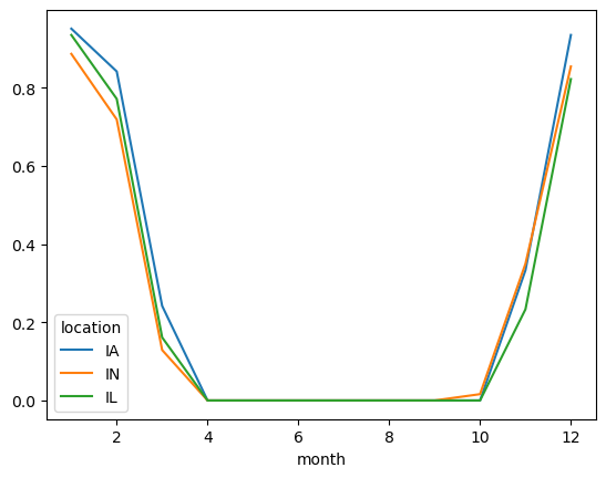
Probability of freeze by calendar month#
[6]:
freeze = (ds["tmin"] <= 0).groupby("time.month").mean("time")
freeze
[6]:
<xarray.DataArray 'tmin' (month: 12, location: 3)>
array([[0.9516129 , 0.88709677, 0.93548387],
       [0.84210526, 0.71929825, 0.77192982],
       [0.24193548, 0.12903226, 0.16129032],
       [0.        , 0.        , 0.        ],
       [0.        , 0.        , 0.        ],
       [0.        , 0.        , 0.        ],
       [0.        , 0.        , 0.        ],
       [0.        , 0.        , 0.        ],
       [0.        , 0.        , 0.        ],
       [0.        , 0.01612903, 0.        ],
       [0.33333333, 0.35      , 0.23333333],
       [0.93548387, 0.85483871, 0.82258065]])
Coordinates:
  * location  (location) <U2 'IA' 'IN' 'IL'
* month (month) int64 1 2 3 4 5 6 7 8 9 10 11 12[7]:
freeze.to_pandas().plot()
[7]:
<AxesSubplot: xlabel='month'>
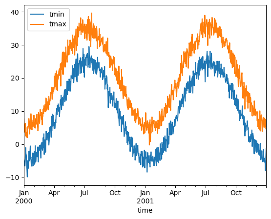
Monthly averaging#
[8]:
monthly_avg = ds.resample(time="1MS").mean()
monthly_avg.sel(location="IA").to_dataframe().plot(style="s-")
[8]:
<AxesSubplot: xlabel='time'>
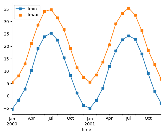
Note that MS here refers to Month-Start; M labels Month-End (the last day of the month).
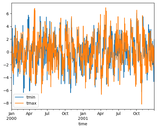
Calculate monthly anomalies#
In climatology, “anomalies” refer to the difference between observations and typical weather for a particular season. Unlike observations, anomalies should not show any seasonal cycle.
[9]:
climatology = ds.groupby("time.month").mean("time")
anomalies = ds.groupby("time.month") - climatology
anomalies.mean("location").to_dataframe()[["tmin", "tmax"]].plot()
[9]:
<AxesSubplot: xlabel='time'>
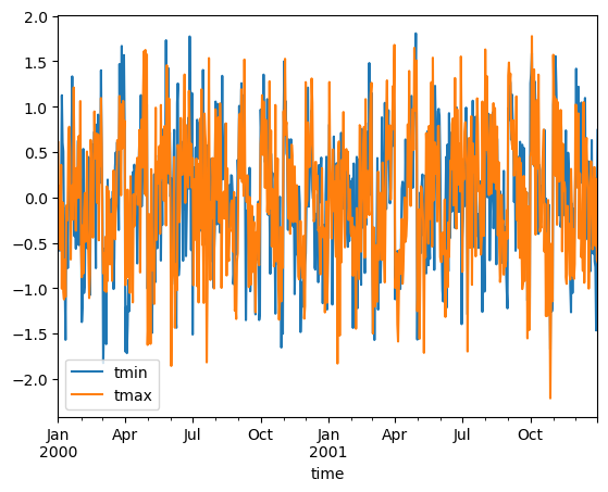
Calculate standardized monthly anomalies#
You can create standardized anomalies where the difference between the observations and the climatological monthly mean is divided by the climatological standard deviation.
[10]:
climatology_mean = ds.groupby("time.month").mean("time")
climatology_std = ds.groupby("time.month").std("time")
stand_anomalies = xr.apply_ufunc(
    lambda x, m, s: (x - m) / s,
    ds.groupby("time.month"),
    climatology_mean,
    climatology_std,
)

stand_anomalies.mean("location").to_dataframe()[["tmin", "tmax"]].plot()
[10]:
<AxesSubplot: xlabel='time'>
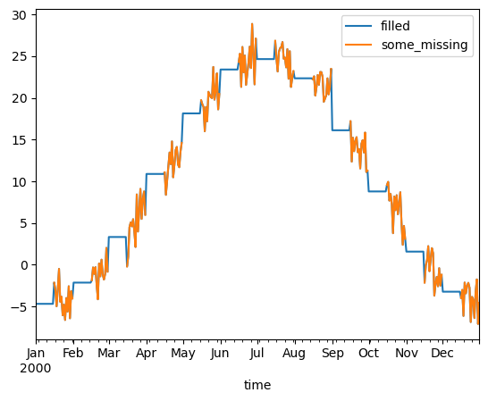
Fill missing values with climatology#
The fillna method on grouped objects lets you easily fill missing values by group:
[11]:
# throw away the first half of every month
some_missing = ds.tmin.sel(time=ds["time.day"] > 15).reindex_like(ds)
filled = some_missing.groupby("time.month").fillna(climatology.tmin)
both = xr.Dataset({"some_missing": some_missing, "filled": filled})
both
[11]:
<xarray.Dataset>
Dimensions:       (time: 731, location: 3)
Coordinates:
  * time          (time) datetime64[ns] 2000-01-01 2000-01-02 ... 2001-12-31
  * location      (location) <U2 'IA' 'IN' 'IL'
    month         (time) int64 1 1 1 1 1 1 1 1 1 ... 12 12 12 12 12 12 12 12 12
Data variables:
    some_missing  (time, location) float64 nan nan nan ... 2.063 -1.346 -4.544
filled (time, location) float64 -5.163 -4.216 ... -1.346 -4.544[12]:
df = both.sel(time="2000").mean("location").reset_coords(drop=True).to_dataframe()
df.head()
[12]:
| some_missing | filled | |
|---|---|---|
| time | ||
| 2000-01-01 | NaN | -4.686763 |
| 2000-01-02 | NaN | -4.686763 |
| 2000-01-03 | NaN | -4.686763 |
| 2000-01-04 | NaN | -4.686763 |
| 2000-01-05 | NaN | -4.686763 |
[13]:
df[["filled", "some_missing"]].plot()
[13]:
<AxesSubplot: xlabel='time'>